39 releases (19 stable)
| 1.10.0 | Feb 21, 2025 |
|---|---|
| 1.9.1 | Dec 17, 2024 |
| 1.9.0 | Sep 28, 2024 |
| 1.6.2 | Jul 23, 2024 |
| 0.1.0 | Jun 22, 2021 |
#30 in Math
88 downloads per month
Used in 9 crates
1.5MB
25K
SLoC
Russell Lab - Scientific laboratory for linear algebra and numerical mathematics
![]()
This crate is part of Russell - Rust Scientific Library
Contents
- Introduction
- Installation
- 🌟 Examples
- Running an example with Intel MKL
- Sorting small tuples
- Check first and second derivatives
- Bessel functions
- Linear fitting
- Chebyshev adaptive interpolation (given function)
- Chebyshev adaptive interpolation (given data)
- Chebyshev adaptive interpolation (given noisy data)
- Lagrange interpolation
- Solution of a 1D PDE using spectral collocation
- Numerical integration: perimeter of ellipse
- Finding a local minimum and a root
- Finding all roots in an interval
- Computing the pseudo-inverse matrix
- Matrix visualization
- Computing eigenvalues and eigenvectors
- Cholesky factorization
- Read a table-formatted data file
- About the column major representation
- Benchmarks
- Notes for developers
Introduction
This library implements specialized mathematical functions (e.g., Bessel, Erf, Gamma) and functions to perform linear algebra computations (e.g., Matrix, Vector, Matrix-Vector, Eigen-decomposition, SVD). This library also implements a set of helpful function for comparing floating-point numbers, measuring computer time, reading table-formatted data, and more.
The code shall be implemented in native Rust code as much as possible. However, light interfaces ("wrappers") are implemented for some of the best tools available in numerical mathematics, including OpenBLAS and Intel MKL.
The code is organized in modules:
algo— algorithms that depend on the other modules (e.g, Lagrange interpolation)base— "base" functionality to help other modulescheck— functions to assist in unit and integration testingmath— mathematical (specialized) functions and constantsmatrix— [NumMatrix] struct and associated functionsmatvec— functions operating on matrices and vectorsvector— [NumVector] struct and associated functions
For linear algebra, the main structures are NumVector and NumMatrix, that are generic Vector and Matrix structures. The Matrix data is stored as column-major. The Vector and Matrix are f64 and Complex64 aliases of NumVector and NumMatrix, respectively.
The linear algebra functions currently handle only (f64, i32) pairs, i.e., accessing the (double, int) C functions. We also consider (Complex64, i32) pairs.
There are many functions for linear algebra, such as (for Real and Complex types):
- Vector addition, copy, inner and outer products, norms, and more
- Matrix addition, multiplication, copy, singular-value decomposition, eigenvalues, pseudo-inverse, inverse, norms, and more
- Matrix-vector multiplication, and more
- Solution of dense linear systems with symmetric or non-symmetric coefficient matrices, and more
- Reading writing files,
linspace, grid generators, Stopwatch, linear fitting, and more - Checking results, comparing floating point numbers, and verifying the correctness of derivatives; see
russell_lab::check
Documentation
External crates
A few other third-party crates related to numerical mathematics and associated disciplines are listed below:
- lambert_w — Computes the Lambert W function
Installation
This crate depends on some non-rust high-performance libraries. See the main README file for the steps to install these dependencies.
Setting Cargo.toml up
![]()
👆 Check the crate version and update your Cargo.toml accordingly:
[dependencies]
russell_lab = "*"
Optional features
The following (Rust) features are available:
intel_mkl: Use Intel MKL instead of OpenBLAS
Note that the main README file presents the steps to compile the required libraries according to each feature.
🌟 Examples
This section illustrates how to use russell_lab. See also:
Running an example with Intel MKL
Consider the following code:
use russell_lab::*;

fn main() -> Result<(), StrError> {
    println!("Using Intel MKL  = {}", using_intel_mkl());
    println!("BLAS num threads = {}", get_num_threads());
    set_num_threads(2);
    println!("BLAS num threads = {}", get_num_threads());
    Ok(())
}
First, run the example without Intel MKL (default):
cargo run --example base_auxiliary_blas
The output looks like this:
Using Intel MKL  = false
BLAS num threads = 24
BLAS num threads = 2
Second, run the code with the intel_mkl feature:
cargo run --example base_auxiliary_blas --features intel_mk
Then, the output looks like this:
Using Intel MKL  = true
BLAS num threads = 24
BLAS num threads = 2
Sorting small tuples
use russell_lab::base::{sort2, sort3, sort4};
use russell_lab::StrError;

fn main() -> Result<(), StrError> {
    // sorting slices with the standard function
    let mut u2 = vec![2.0, 1.0];
    let mut u3 = vec![3.0, 1.0, 2.0];
    let mut u4 = vec![3.0, 1.0, 4.0, 2.0];
    u2.sort_by(|a, b| a.partial_cmp(b).unwrap());
    u3.sort_by(|a, b| a.partial_cmp(b).unwrap());
    u4.sort_by(|a, b| a.partial_cmp(b).unwrap());
    println!("u2 = {:?}", u2);
    println!("u3 = {:?}", u3);
    println!("u4 = {:?}", u4);
    assert_eq!(&u2, &[1.0, 2.0]);
    assert_eq!(&u3, &[1.0, 2.0, 3.0]);
    assert_eq!(&u4, &[1.0, 2.0, 3.0, 4.0]);

    // sorting small tuples
    let mut v2 = (2.0, 1.0);
    let mut v3 = (3.0, 1.0, 2.0);
    let mut v4 = (3.0, 1.0, 4.0, 2.0);
    sort2(&mut v2);
    sort3(&mut v3);
    sort4(&mut v4);
    println!("v2 = {:?}", v2);
    println!("v3 = {:?}", v3);
    println!("v4 = {:?}", v4);
    assert_eq!(v2, (1.0, 2.0));
    assert_eq!(v3, (1.0, 2.0, 3.0));
    assert_eq!(v4, (1.0, 2.0, 3.0, 4.0));
    Ok(())
}
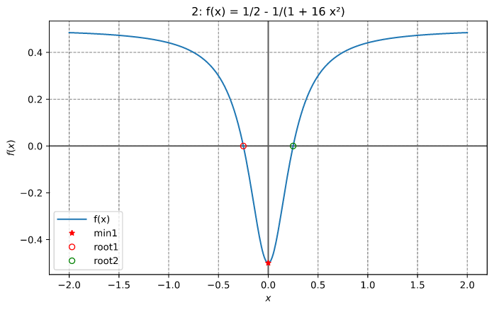
Check first and second derivatives
Check the implementation of the first and second derivatives of f(x) (illustrated below).
use russell_lab::algo::NoArgs;
use russell_lab::check::{deriv1_approx_eq, deriv2_approx_eq};
use russell_lab::{StrError, Vector};

fn main() -> Result<(), StrError> {
    // f(x)
    let f = |x: f64, _: &mut NoArgs| Ok(1.0 / 2.0 - 1.0 / (1.0 + 16.0 * x * x));

    // g(x) = df/dx(x)
    let g = |x: f64, _: &mut NoArgs| Ok((32.0 * x) / f64::powi(1.0 + 16.0 * f64::powi(x, 2), 2));

    // h(x) = d²f/dx²(x)
    let h = |x: f64, _: &mut NoArgs| {
        Ok((-2048.0 * f64::powi(x, 2)) / f64::powi(1.0 + 16.0 * f64::powi(x, 2), 3)
            + 32.0 / f64::powi(1.0 + 16.0 * f64::powi(x, 2), 2))
    };

    let xx = Vector::linspace(-2.0, 2.0, 9)?;
    let args = &mut 0;
    println!("{:>4}{:>23}{:>23}", "x", "df/dx", "d²f/dx²");
    for x in xx {
        let dfdx = g(x, args)?;
        let d2dfx2 = h(x, args)?;
        println!("{:>4}{:>23}{:>23}", x, dfdx, d2dfx2);
        deriv1_approx_eq(dfdx, x, args, 1e-10, f);
        deriv2_approx_eq(d2dfx2, x, args, 1e-9, f);
    }
    Ok(())
}
Output:
   x                  df/dx                d²f/dx²
  -2   -0.01514792899408284  -0.022255803368229403
-1.5   -0.03506208911614317   -0.06759718081851025
  -1   -0.11072664359861592   -0.30612660289029103
-0.5                  -0.64                 -2.816
   0                      0                     32
 0.5                   0.64                 -2.816
   1    0.11072664359861592   -0.30612660289029103
 1.5    0.03506208911614317   -0.06759718081851025
   2    0.01514792899408284  -0.022255803368229403
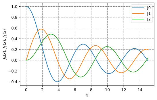
Bessel functions
Plotting the Bessel J0, J1, and J2 functions:
use plotpy::{Curve, Plot};
use russell_lab::math::{bessel_j0, bessel_j1, bessel_jn, GOLDEN_RATIO};
use russell_lab::{StrError, Vector};

const OUT_DIR: &str = "/tmp/russell_lab/";

fn main() -> Result<(), StrError> {
    // values
    let xx = Vector::linspace(0.0, 15.0, 101)?;
    let j0 = xx.get_mapped(|x| bessel_j0(x));
    let j1 = xx.get_mapped(|x| bessel_j1(x));
    let j2 = xx.get_mapped(|x| bessel_jn(2, x));
    // plot
    if false { // <<< remove this condition
    let mut curve_j0 = Curve::new();
    let mut curve_j1 = Curve::new();
    let mut curve_j2 = Curve::new();
    curve_j0.set_label("J0").draw(xx.as_data(), j0.as_data());
    curve_j1.set_label("J1").draw(xx.as_data(), j1.as_data());
    curve_j2.set_label("J2").draw(xx.as_data(), j2.as_data());
    let mut plot = Plot::new();
    let path = format!("{}/math_bessel_functions_1.svg", OUT_DIR);
    plot.add(&curve_j0)
        .add(&curve_j1)
        .add(&curve_j2)
        .grid_labels_legend("$x$", "$J_0(x),\\,J_1(x),\\,J_2(x)$")
        .set_figure_size_points(GOLDEN_RATIO * 280.0, 280.0)
        .save(&path)?;
    }
    Ok(())
}
Output:
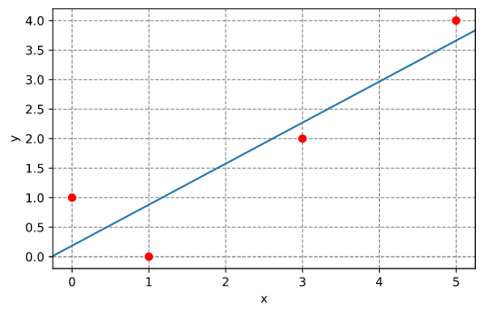
Linear fitting
Fit a line through a set of points. The line has slope m and intercepts the y axis at x=0 with y(x=0) = c.
use russell_lab::algo::linear_fitting;
use russell_lab::{approx_eq, StrError};

fn main() -> Result<(), StrError> {
    // model: c is the y value @ x = 0; m is the slope
    let x = [0.0, 1.0, 3.0, 5.0];
    let y = [1.0, 0.0, 2.0, 4.0];
    let (c, m) = linear_fitting(&x, &y, false)?;
    println!("c = {}, m = {}", c, m);
    approx_eq(c, 0.1864406779661015, 1e-15);
    approx_eq(m, 0.6949152542372882, 1e-15);
    Ok(())
}
Results:
Chebyshev adaptive interpolation (given function)
This example illustrates the use of InterpChebyshev to interpolate data given a function.
Results:
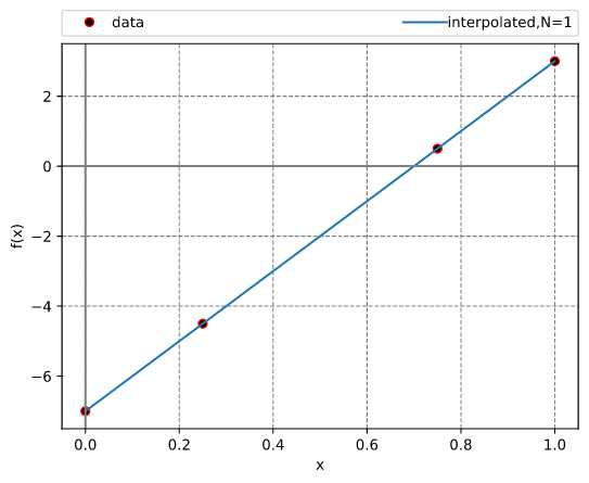
Chebyshev adaptive interpolation (given data)
This example illustrates the use of InterpChebyshev to interpolate discrete data.
Results:
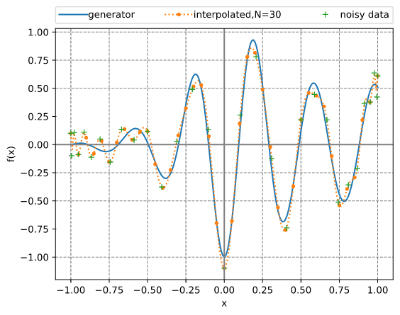
Chebyshev adaptive interpolation (given noisy data)
This example illustrates the use of InterpChebyshev to interpolate noisy data.
Results:
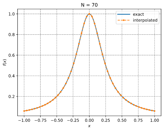
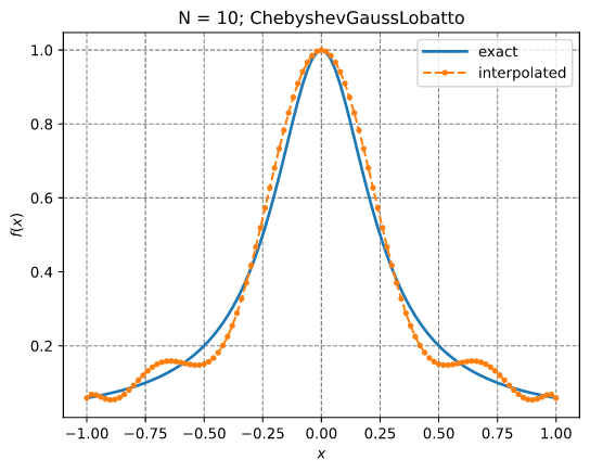
Lagrange interpolation
This example illustrates the use of InterpLagrange with at Chebyshev-Gauss-Lobatto grid to interpolate Runge's equation.
Results:
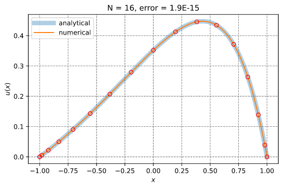
Solution of a 1D PDE using spectral collocation
This example illustrates the solution of a 1D PDE using the spectral collocation method. It employs the InterpLagrange struct.
d²u     du          x
——— - 4 —— + 4 u = e  + C
dx²     dx

    -4 e
C = ——————
    1 + e²

x ∈ [-1, 1]
Boundary conditions:
u(-1) = 0 and u(1) = 0
Reference solution:
        x   sinh(1)  2x   C
u(x) = e  - ——————— e   + —
            sinh(2)       4
Results:
Numerical integration: perimeter of ellipse
use russell_lab::algo::Quadrature;
use russell_lab::math::{elliptic_e, PI};
use russell_lab::{approx_eq, StrError};

fn main() -> Result<(), StrError> {
    //  Determine the perimeter P of an ellipse of length 2 and width 1
    //
    //      2π
    //     ⌠   ____________________
    // P = │ \╱ ¼ sin²(θ) + cos²(θ)  dθ
    //     ⌡
    //    0

    let mut quad = Quadrature::new();
    let args = &mut 0;
    let (perimeter, _) = quad.integrate(0.0, 2.0 * PI, args, |theta, _| {
        Ok(f64::sqrt(
            0.25 * f64::powi(f64::sin(theta), 2) + f64::powi(f64::cos(theta), 2),
        ))
    })?;
    println!("\nperimeter = {}", perimeter);

    // complete elliptic integral of the second kind E(0.75)
    let ee = elliptic_e(PI / 2.0, 0.75)?;

    // reference solution
    let ref_perimeter = 4.0 * ee;
    approx_eq(perimeter, ref_perimeter, 1e-14);
    Ok(())
}
Finding a local minimum and a root
This example finds the local minimum between 0.1 and 0.3 and the root between 0.3 and 0.4 for the function illustrated below
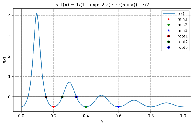
The output looks like:
x_optimal = 0.20000000003467466

Number of function evaluations   = 18
Number of Jacobian evaluations   = 0
Number of iterations             = 18
Error estimate                   = unavailable
Total computation time           = 6.11µs

x_root = 0.3397874957748173

Number of function evaluations   = 10
Number of Jacobian evaluations   = 0
Number of iterations             = 9
Error estimate                   = unavailable
Total computation time           = 907ns
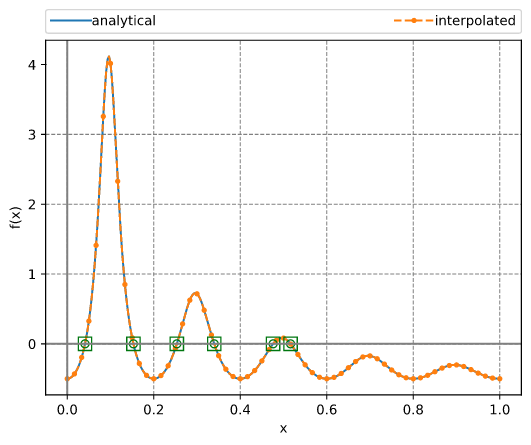
Finding all roots in an interval
This example employs a Chebyshev interpolant to find all roots of a function in an interval. The method uses adaptive interpolation followed by calculating the eigenvalues of the companion matrix. These eigenvalues equal the roots of the polynomial. After that, a simple Newton refining (polishing) algorithm is applied.
The output looks like:
N = 184
roots =
┌                     ┐
│ 0.04109147217011577 │
│  0.1530172326889439 │
│ 0.25340124027487965 │
│ 0.33978749525956276 │
│ 0.47590538542276967 │
│  0.5162732673126048 │
└                     ┘
f @ roots =
┌           ┐
│  1.84E-08 │
│ -1.51E-08 │
│ -2.40E-08 │
│  9.53E-09 │
│ -1.16E-08 │
│ -5.80E-09 │
└           ┘
refined roots =
┌                     ┐
│ 0.04109147155278252 │
│ 0.15301723213859994 │
│ 0.25340124149692184 │
│   0.339787495774806 │
│ 0.47590538689192813 │
│  0.5162732665558162 │
└                     ┘
f @ refined roots =
┌           ┐
│  6.66E-16 │
│ -2.22E-16 │
│ -2.22E-16 │
│  1.33E-15 │
│  4.44E-16 │
│ -2.22E-16 │
└           ┘
The function and the roots are illustrated in the figure below.
References
- Boyd JP (2002) Computing zeros on a real interval through Chebyshev expansion and polynomial rootfinding, SIAM Journal of Numerical Analysis, 40(5):1666-1682
- Boyd JP (2013) Finding the zeros of a univariate equation: proxy rootfinders, Chebyshev interpolation, and the companion matrix, SIAM Journal of Numerical Analysis, 55(2):375-396.
- Boyd JP (2014) Solving Transcendental Equations: The Chebyshev Polynomial Proxy and Other Numerical Rootfinders, Perturbation Series, and Oracles, SIAM, pp460
Computing the pseudo-inverse matrix
use russell_lab::{mat_pseudo_inverse, Matrix, StrError};

fn main() -> Result<(), StrError> {
    // set matrix
    let mut a = Matrix::from(&[
      [1.0, 0.0], //
      [0.0, 1.0], //
      [0.0, 1.0], //
    ]);
    let a_copy = a.clone();

    // compute pseudo-inverse matrix
    let mut ai = Matrix::new(2, 3);
    mat_pseudo_inverse(&mut ai, &mut a)?;

    // compare with solution
    let ai_correct = "┌                ┐\n\
                      │ 1.00 0.00 0.00 │\n\
                      │ 0.00 0.50 0.50 │\n\
                      └                ┘";
    assert_eq!(format!("{:.2}", ai), ai_correct);

    // compute a ⋅ ai
    let (m, n) = a.dims();
    let mut a_ai = Matrix::new(m, m);
    for i in 0..m {
        for j in 0..m {
            for k in 0..n {
                a_ai.add(i, j, a_copy.get(i, k) * ai.get(k, j));
            }
        }
    }

    // check: a ⋅ ai ⋅ a = a
    let mut a_ai_a = Matrix::new(m, n);
    for i in 0..m {
        for j in 0..n {
            for k in 0..m {
                a_ai_a.add(i, j, a_ai.get(i, k) * a_copy.get(k, j));
            }
        }
    }
    let a_ai_a_correct = "┌           ┐\n\
                          │ 1.00 0.00 │\n\
                          │ 0.00 1.00 │\n\
                          │ 0.00 1.00 │\n\
                          └           ┘";
    assert_eq!(format!("{:.2}", a_ai_a), a_ai_a_correct);
    Ok(())
}
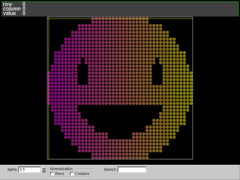
Matrix visualization
We can use the fantastic tool named vismatrix to visualize the pattern of non-zero values of a matrix. With vismatrix, we can click on each circle and investigate the numeric values as well.
The function mat_write_vismatrix writes the input data file for vismatrix.
After generating the "dot-smat" file, run the following command:
vismatrix /tmp/russell_lab/matrix_visualization.smat
Output:
Computing eigenvalues and eigenvectors
use russell_lab::*;

fn main() -> Result<(), StrError> {
    // set matrix
    let data = [[2.0, 0.0, 0.0], [0.0, 3.0, 4.0], [0.0, 4.0, 9.0]];
    let mut a = Matrix::from(&data);

    // allocate output arrays
    let m = a.nrow();
    let mut l_real = Vector::new(m);
    let mut l_imag = Vector::new(m);
    let mut v_real = Matrix::new(m, m);
    let mut v_imag = Matrix::new(m, m);

    // perform the eigen-decomposition
    mat_eigen(&mut l_real, &mut l_imag, &mut v_real, &mut v_imag, &mut a)?;

    // check results
    assert_eq!(
        format!("{:.1}", l_real),
        "┌      ┐\n\
         │ 11.0 │\n\
         │  1.0 │\n\
         │  2.0 │\n\
         └      ┘"
    );
    assert_eq!(
        format!("{}", l_imag),
        "┌   ┐\n\
         │ 0 │\n\
         │ 0 │\n\
         │ 0 │\n\
         └   ┘"
    );

    // check eigen-decomposition (similarity transformation) of a
    // symmetric matrix with real-only eigenvalues and eigenvectors
    let a_copy = Matrix::from(&data);
    let lam = Matrix::diagonal(l_real.as_data());
    let mut a_v = Matrix::new(m, m);
    let mut v_l = Matrix::new(m, m);
    let mut err = Matrix::filled(m, m, f64::MAX);
    mat_mat_mul(&mut a_v, 1.0, &a_copy, &v_real, 0.0)?;
    mat_mat_mul(&mut v_l, 1.0, &v_real, &lam, 0.0)?;
    mat_add(&mut err, 1.0, &a_v, -1.0, &v_l)?;
    approx_eq(mat_norm(&err, Norm::Max), 0.0, 1e-15);
    Ok(())
}
Cholesky factorization
use russell_lab::*;

fn main() -> Result<(), StrError> {
    // set matrix
    let sym = 0.0;
    #[rustfmt::skip]
    let mut a = Matrix::from(&[
        [  4.0,   sym,   sym],
        [ 12.0,  37.0,   sym],
        [-16.0, -43.0,  98.0],
    ]);

    // perform factorization
    mat_cholesky(&mut a, false)?;

    // define alias (for convenience)
    let l = &a;

    // compare with solution
    let l_correct = "┌          ┐\n\
                     │  2  0  0 │\n\
                     │  6  1  0 │\n\
                     │ -8  5  3 │\n\
                     └          ┘";
    assert_eq!(format!("{}", l), l_correct);

    // check:  l ⋅ lᵀ = a
    let m = a.nrow();
    let mut l_lt = Matrix::new(m, m);
    for i in 0..m {
        for j in 0..m {
            for k in 0..m {
                l_lt.add(i, j, l.get(i, k) * l.get(j, k));
            }
        }
    }
    let l_lt_correct = "┌             ┐\n\
                        │   4  12 -16 │\n\
                        │  12  37 -43 │\n\
                        │ -16 -43  98 │\n\
                        └             ┘";
    assert_eq!(format!("{}", l_lt), l_lt_correct);
    Ok(())
}
Read a table-formatted data file
The goal is to read the following file (clay-data.txt):
# Fujinomori clay test results

     sr        ea        er   # header
1.00000  -6.00000   0.10000
2.00000   7.00000   0.20000
3.00000   8.00000   0.20000   # << look at this line

# comments plus new lines are OK

4.00000   9.00000   0.40000
5.00000  10.00000   0.50000

# bye
The code below illustrates how to do it.
Each column (sr, ea, er) is accessible via the get method of the [HashMap].
use russell_lab::{read_table, StrError};
use std::collections::HashMap;
use std::env;
use std::path::PathBuf;

fn main() -> Result<(), StrError> {
    // get the asset's full path
    let root = PathBuf::from(env::var("CARGO_MANIFEST_DIR").unwrap());
    let full_path = root.join("data/tables/clay-data.txt");

    // read the file
    let labels = &["sr", "ea", "er"];
    let table: HashMap<String, Vec<f64>> = read_table(&full_path, Some(labels))?;

    // check the columns
    assert_eq!(table.get("sr").unwrap(), &[1.0, 2.0, 3.0, 4.0, 5.0]);
    assert_eq!(table.get("ea").unwrap(), &[-6.0, 7.0, 8.0, 9.0, 10.0]);
    assert_eq!(table.get("er").unwrap(), &[0.1, 0.2, 0.2, 0.4, 0.5]);
    Ok(())
}
About the column major representation
Only the COL-MAJOR representation is considered here.
    ┌     ┐  row_major = {0, 3,
    │ 0 3 │               1, 4,
A = │ 1 4 │               2, 5};
    │ 2 5 │
    └     ┘  col_major = {0, 1, 2,
    (m × n)               3, 4, 5}

Aᵢⱼ = col_major[i + j·m] = row_major[i·n + j]
        ↑
COL-MAJOR IS ADOPTED HERE
The main reason to use the col-major representation is to make the code work better with BLAS/LAPACK written in Fortran. Although those libraries have functions to handle row-major data, they usually add an overhead due to temporary memory allocation and copies, including transposing matrices. Moreover, the row-major versions of some BLAS/LAPACK libraries produce incorrect results (notably the DSYEV).
Benchmarks
Need to install:
cargo install cargo-criterion
Run the benchmarks with:
bash ./zscripts/benchmark.bash
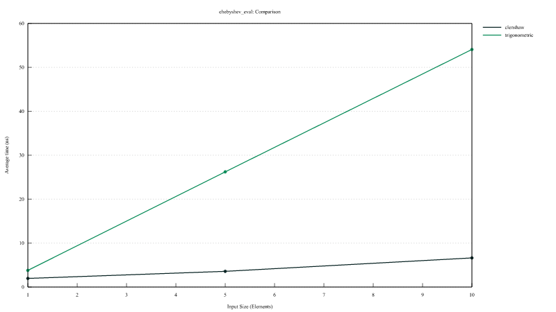
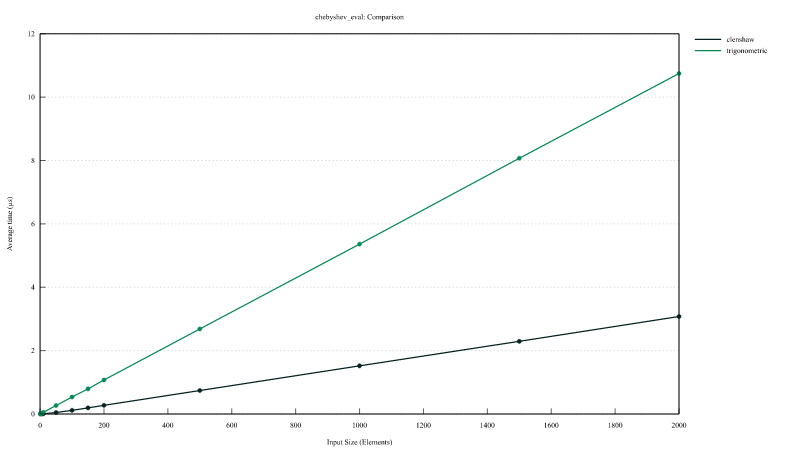
Chebyshev polynomial evaluation
Comparison of the performances of InterpChebyshev::eval implementing the Clenshaw algorithm and InterpChebyshev::eval_using_trig using the trigonometric functions.
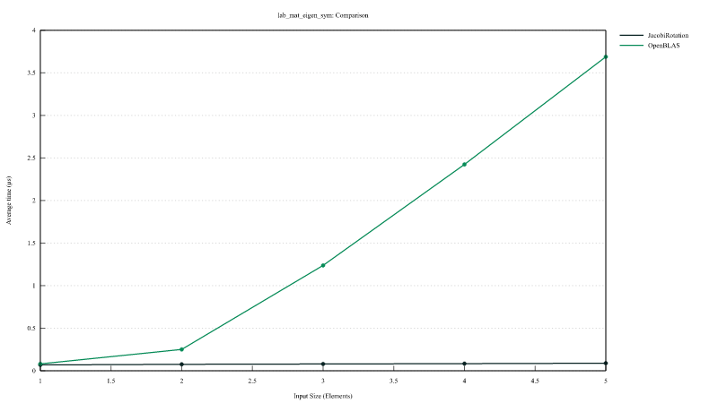
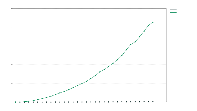
Jacobi Rotation versus LAPACK DSYEV
Comparison of the performances of mat_eigen_sym_jacobi (Jacobi rotation) versus mat_eigen_sym (calling LAPACK DSYEV).
Notes for developers
- The
c_codedirectory contains a thin wrapper to the BLAS libraries (OpenBLAS or Intel MKL) - The
c_codedirectory also contains a wrapper to the C math functions - The
build.rsfile uses the crateccto build the C-wrappers