3 releases (breaking)

0.3.0	Oct 15, 2023
0.2.1	Jul 30, 2023
0.1.0	Feb 1, 2022

#704 in Math

35 downloads per month

MIT license

1.5MB
7.5K SLoC

Porous Media Simulator using the Finite Element Method

🚧 Work in progress...

Introduction
Installation
Setting Cargo.toml
Examples

Introduction

This code implements simulator using the finite element method for the behavior of solids, structures, and porous media.

See the documentation for further information:

pmsim documentation - Contains the API reference and examples

Installation

This crates depends on russell_lab and, hence, needs some external libraries. See the installation of required dependencies on russell_lab.

Setting Cargo.toml

👆 Check the crate version and update your Cargo.toml accordingly:

[dependencies]
gemlab = "*"

Examples

For all simulations:

Legend:
✅ : converged
👍 : converging
🥵 : diverging
😱 : found NaN or Inf
❋  : non-scaled max(R)
?  : no info abut convergence

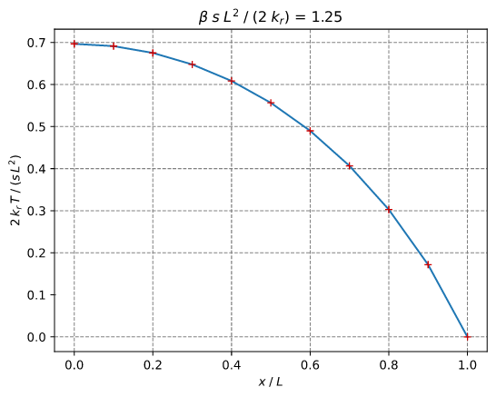
Heat: Arpaci Nonlinear 1d

Arpaci's Example 3-8 on page 130 (variable conductivity)

Arpaci V. S. (1966) Conduction Heat Transfer, Addison-Wesley, 551p

Test goal

This tests verifies the nonlinear solver for the diffusion equation with a variable conductivity coefficient.

Mesh

Initial conditions

Temperature T = 0 at all points

Boundary conditions

Temperature T = 0 on right side @ x = L

Configuration and parameters

Steady simulation
Source = 5
Variable conductivity (k = (1 + β T) kᵣ I) with kᵣ = 2

Note

The temperature at the right T = 0 (T_inf) must be zero in order to result in k(T_inf) = kᵣ as required by the analytical solution.

Simulation and results

heat_arpaci_nonlinear_1d.rs

                                                  _   
timestep             t            Δt  iter    max(R)  
       1   1.000000e-1   1.000000e-1     .        .  
       .             .             .     1    2.50e0❋ 
       .             .             .     2    1.28e0? 
       .             .             .     3   9.36e-2👍
       .             .             .     4   1.25e-3👍
       .             .             .     5   1.42e-7👍
       .             .             .     6  1.35e-14✅

T(0) = 87.08286933869708  (87.08286933869707)

The figure below compares the numerical with the analytical results.

Results

Heat: Bhatti Example 1.5 Convection

Bhatti's Example 1.5 on page 28

Bhatti, M.A. (2005) Fundamental Finite Element Analysis and Applications, Wiley, 700p.

Test goal

This test verifies the steady heat equation with prescribed temperature and convection

Mesh

Boundary conditions

Convection Cc = (27, 20) on the right edge
Prescribed temperature T = 300 on the left edge

Configuration and parameters

Steady simulation
No source
Constant conductivity kx = ky = 1.4

Simulation and results

heat_bhatti_1d5_convection.rs

                                                  _   
timestep             t            Δt  iter    max(R)  
       1   1.000000e-1   1.000000e-1     .        .  
       .             .             .     1    1.05e3❋ 
       .             .             .     2  1.71e-15✅

Heat: Bhatti Example 6.22 Convection

Bhatti's Example 6.22 on page 449

Bhatti, M.A. (2005) Fundamental Finite Element Analysis and Applications, Wiley, 700p.

Test goal

This test verifies the steady heat equation with prescribed temperature, convection, flux, and a volumetric source term. Also, it checks the use of Qua8 elements.

Mesh

Boundary conditions (see page 445)

Flux Qt = 8,000 on left side, edge (0,10,11)
Convection Cc = (55, 20) on top edges (0,2,1), (2,4,3), and (4,6,5)
Prescribed temperature T = 110 on the bottom edge (8,10,9)

Configuration and parameters

Steady simulation
Source = 5e6 over the region
Constant conductivity kx = ky = 45

Simulation and results

heat_bhatti_6d22_convection.rs

                                                  _   
timestep             t            Δt  iter    max(R)  
       1   1.000000e-1   1.000000e-1     .        .  
       .             .             .     1    3.09e4❋ 
       .             .             .     2  6.09e-16✅

Heat: Lewis Example 6.4.2 Transient 1d

Lewis' Example 6.4.2 on page 159

Lewis R, Nithiarasu P, and Seetharamu KN (2004) Fundamentals of the Finite Element Method for Heat and Fluid Flow, Wiley, 341p

Test goal

This test verifies the transient diffusion in 1D

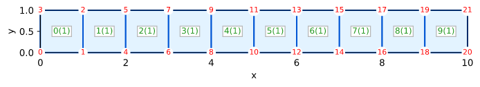
Mesh

o-----------------------------------------------------------o
|    |    |    |    |    |    |    |    |    |    .....     | h = 1
o-----------------------------------------------------------o
                     <-  L = 20 ->

Mesh

Initial conditions

Temperature T = 0 at all points

Boundary conditions

Flux Qt = 1 on left side @ x = 0

Configuration and parameters

Transient simulation
No source
Constant conductivity kx = ky = 1
Coefficient ρ = 1

Simulation and results

heat_lewis_transient_1d.rs

                                                  _   
timestep             t            Δt  iter    max(R)  
       1   1.000000e-1   1.000000e-1     .        .  
       .             .             .     1   6.67e-1❋ 
       .             .             .     2  2.36e-16✅
       2   2.000000e-1   1.000000e-1     .        .  
       .             .             .     1    1.24e0❋ 
       .             .             .     2  6.07e-16✅
       3   3.000000e-1   1.000000e-1     .        .  
       .             .             .     1    1.08e0❋ 
       .             .             .     2  2.55e-16✅
       4   4.000000e-1   1.000000e-1     .        .  
       .             .             .     1   9.73e-1❋ 
       .             .             .     2  3.38e-16✅
       5   5.000000e-1   1.000000e-1     .        .  
       .             .             .     1   8.94e-1❋ 
       .             .             .     2  3.25e-16✅
       6   6.000000e-1   1.000000e-1     .        .  
       .             .             .     1   8.33e-1❋ 
       .             .             .     2  4.24e-16✅
       7   7.000000e-1   1.000000e-1     .        .  
       .             .             .     1   7.84e-1❋ 
       .             .             .     2  6.89e-16✅
       8   8.000000e-1   1.000000e-1     .        .  
       .             .             .     1   7.44e-1❋ 
       .             .             .     2  4.46e-16✅
       9   9.000000e-1   1.000000e-1     .        .  
       .             .             .     1   7.09e-1❋ 
       .             .             .     2  5.85e-16✅
      10    1.000000e0   1.000000e-1     .        .  
       .             .             .     1   6.79e-1❋ 
       .             .             .     2  1.03e-15✅

point = 0, x = 0.00, T = 1.105099, diff = 2.3280e-2
point = 3, x = 0.00, T = 1.105099, diff = 2.3280e-2
point = 7, x = 0.00, T = 1.105099, diff = 2.3280e-2
point = 4, x = 1.00, T = 0.376835, diff = 2.2447e-2
point = 6, x = 1.00, T = 0.376835, diff = 2.2447e-2
point = 1, x = 2.00, T = 0.085042, diff = 1.5467e-2
point = 2, x = 2.00, T = 0.085042, diff = 1.5467e-2

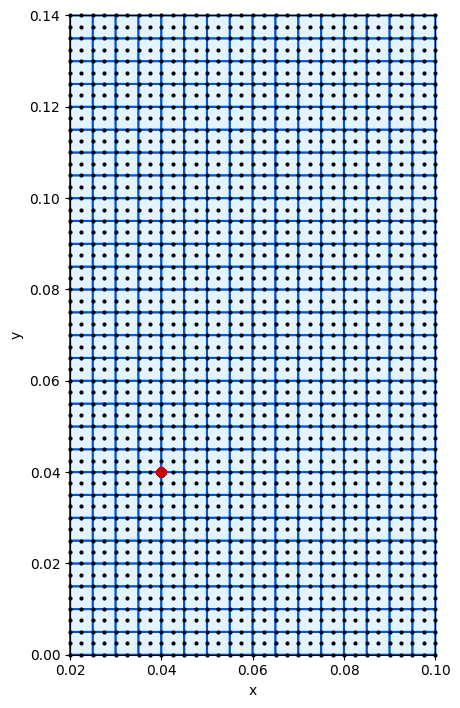
Heat: Mathematica Axisymmetric Nafems

From Mathematica Heat Transfer Model Verification Tests (HeatTransfer-FEM-Stationary-2DAxisym-Single-HeatTransfer-0002)

NAFEMS benchmark test

https://reference.wolfram.com/language/PDEModels/tutorial/HeatTransfer/HeatTransferVerificationTests.html

Test goal

This test verifies the steady heat equation with a localized flux boundary condition

MESH (not-to-scale, not-equal-axis)

0.14     ||++++++++++++++++++++++++
         ||   |    |    |    |    +
         ||-----------------------+
         ||   |    |    |    |    +
0.10  →→ |------------------------+  yb
      →→ |    |    |    |    |    +
      →→ |------------------------+
      →→ |    |    |    |    |    +
      →→ |------------------------+
      →→ |    |    |    |    |    +
0.04  →→ |--------(#)-------------+  ya
         ||   |    |    |    |    +
         ||-----------------------+
         ||   |    |    |    |    +
0.00     ||++++++++++++++++++++++++
        0.02     0.04            0.10
        rin      rref            rout

'+' indicates sides with T = 273.15
|| means insulated
→→ means flux with Qt = 5e5
(#) indicates a reference point to check the results

Mesh

Initial conditions

Temperature T = 0 at all points

Boundary conditions

Temperature T = 273.15 on the top, bottom, and right edges
Flux Qt = 5e5 on the middle-left edges from y=0.04 to y=0.10

Configuration and parameters

Steady simulation
No source
Constant conductivity kx = ky = 52

Simulation and results

heat_mathematica_axisym_nafems.rs

                                                  _   
timestep             t            Δt  iter    max(R)  
       1   1.000000e-1   1.000000e-1     .        .  
       .             .             .     1    4.45e3❋ 
       .             .             .     2  3.23e-12✅

T = 332.9704335048643, reference = 332.97, rel_error = 0.00013019 %

Heat: Mathematica Axisymmetric Simple

From Mathematica Heat Transfer Model Verification Tests (HeatTransfer-FEM-Stationary-2DAxisym-Single-HeatTransfer-0001)

2D Axisymmetric Single Equation

https://reference.wolfram.com/language/PDEModels/tutorial/HeatTransfer/HeatTransferVerificationTests.html

Test goal

This test verifies the steady heat equation in 1D with prescribed flux

Mesh

  →→ ---------------------
  →→ |    |    |    |    |  h
  →→ ---------------------
    1.0                 2.0
    rin                rout

Mesh

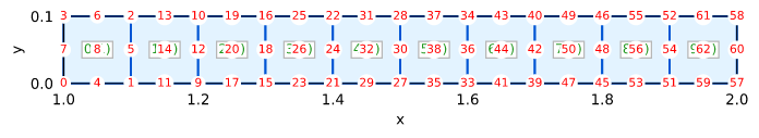
Initial conditions

Temperature T = 0 at all points

Boundary conditions

Temperature T = 10.0 on the right edge
Flux Qt = 100.0 on the left edge

Configuration and parameters

Steady simulation
No source
Constant conductivity kx = ky = 10.0

Simulation and results

heat_mathematica_axisym_simple.rs

                                                  _   
timestep             t            Δt  iter    max(R)  
       1   1.000000e-1   1.000000e-1     .        .  
       .             .             .     1    3.51e2❋ 
       .             .             .     2  3.55e-13✅

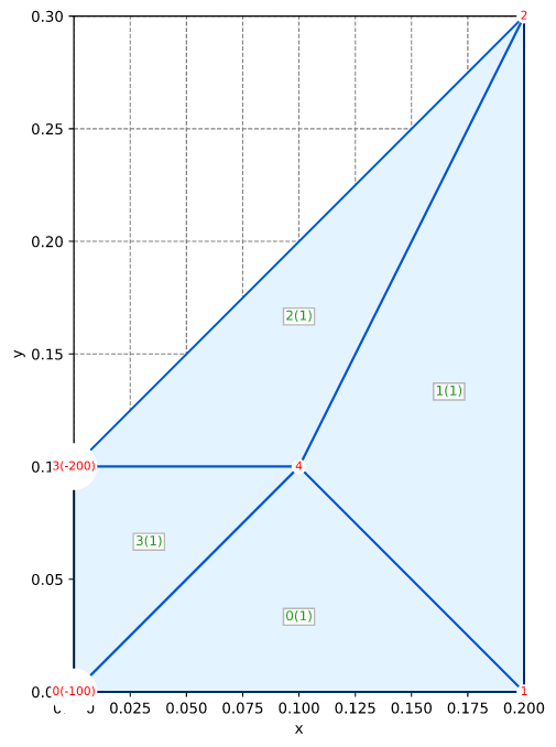
Rod: Bhatti Example 1.4 Truss

Bhatti's Example 1.4 on page 25

Bhatti, M.A. (2005) Fundamental Finite Element Analysis and Applications, Wiley, 700p.

Test goal

This test verifies a 2D frame with rod elements and concentrated forces

Mesh

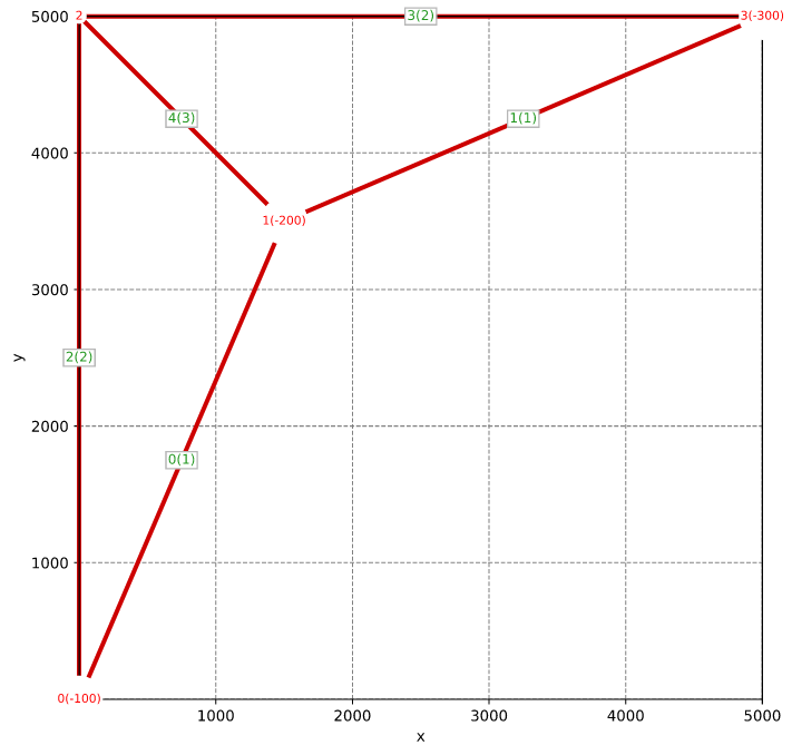
Boundary conditions

Fully fixed @ points 0 and 3
Concentrated load @ point 1 with Fy = -150,000

Configuration and parameters

Static simulation
Attribute 1: Area = 4,000; Young = 200,000
Attribute 2: Area = 3,000; Young = 200,000
Attribute 3: Area = 2,000; Young = 70,000

Simulation and results

rod_bhatti_1d4_truss.rs

                                                  _   
timestep             t            Δt  iter    max(R)  
       1   1.000000e-1   1.000000e-1     .        .  
       .             .             .     1    1.50e5❋ 
       .             .             .     2  1.46e-11✅

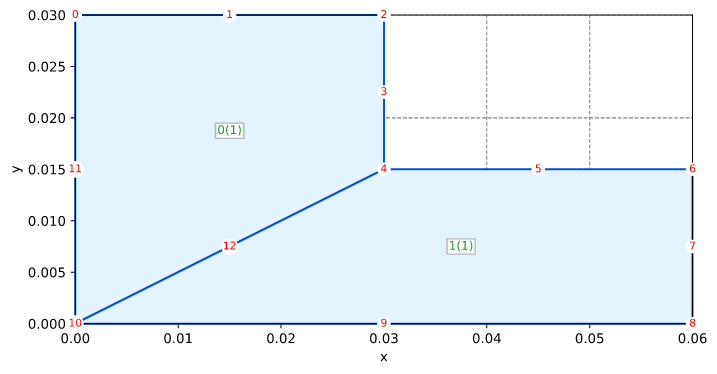
Solid Bhatti Example 1.6 Plane Stress

Bhatti's Example 1.6 on page 32

Bhatti, M.A. (2005) Fundamental Finite Element Analysis and Applications, Wiley, 700p.

Test goal

This test verifies the equilibrium of a thin bracket modelled by assuming plane-stress

Mesh

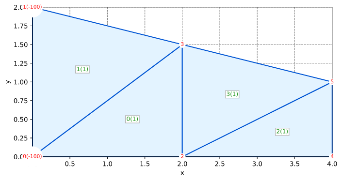
Boundary conditions

Fully fixed @ points 0 and 1
Distributed load along edges (1,3) and (3,5) with Qn = -20

Configuration and parameters

Static simulation
Young = 10,000
Poisson = 0.2
Plane-stress with thickness = 0.25

Simulation and results

solid_bhatti_1d6_plane_stress.rs

                                                  _   
timestep             t            Δt  iter    max(R)  
       1   1.000000e-1   1.000000e-1     .        .  
       .             .             .     1    1.00e1❋ 
       .             .             .     2  3.91e-14✅

Solid Felippa Thick Cylinder Axisymmetric

Felippa's Benchmark 14.1 (Figure 14.1) on page 14-3

Felippa C, Advanced Finite Elements

Test goal

This test verifies the axisymmetric modelling of a chick cylindrical tube under internal pressure. There is an analytical solution, developed for the plane-strain case. However, this tests employs the AXISYMMETRIC representation.

Mesh

            Uy FIXED
 →o------o------o------o------o
 →|      |   .......   |      |
 →o------o------o------o------o
            Uy FIXED

Boundary conditions

Fix bottom edge vertically
Fix top edge vertically
Distributed load Qn = -PRESSURE on left edge

Configuration and parameters

Static simulation
Young = 1000, Poisson = 0.0
Axisymmetric
NOTE: using 4 integration points because it gives better results with Qua8

Simulation and results

solid_felippa_thick_cylinder_axisym.rs

                                                  _   
timestep             t            Δt  iter    max(R)  
       1   1.000000e-1   1.000000e-1     .        .  
       .             .             .     1    5.33e1❋ 
       .             .             .     2  3.16e-13✅

point = 0, r = 4.0, Ux = 0.055238095238095454, diff = 2.1510571102112408e-16
point = 1, r = 7.0, Ux = 0.040544217687075015, diff = 1.8735013540549517e-16
point = 4, r = 5.5, Ux = 0.04510822510822529, diff = 1.8041124150158794e-16
point = 8, r = 10.0, Ux = 0.03809523809523828, diff = 1.8041124150158794e-16
point = 10, r = 8.5, Ux = 0.03859943977591054, diff = 1.8041124150158794e-16

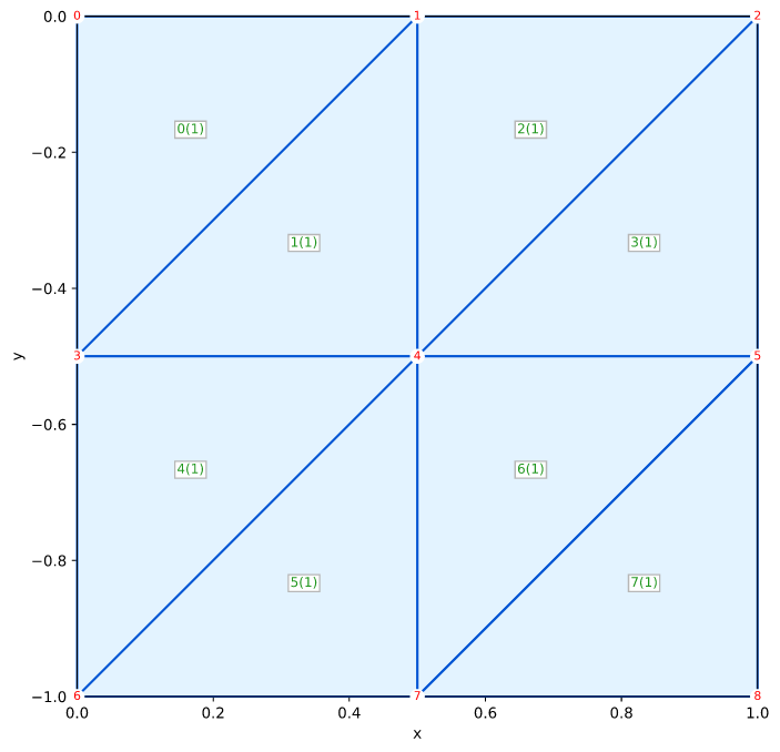
Solid Smith Figure 5.2 Tri3 Plane Strain

Smith's Example 5.2 (Figure 5.2) on page 173

Smith IM, Griffiths DV, and Margetts L (2014) Programming the Finite Element Method, Wiley, Fifth Edition, 664p

Test goal

This test verifies a plane-strain simulation with Tri3 elements

Mesh

              1.0 kN/m²
        ↓↓↓↓↓↓↓↓↓↓↓↓↓↓↓↓↓↓↓↓↓
 0.0   ▷0---------1---------2
        |       ,'|       ,'|   E = 1e6 kN/m²
        |  0  ,'  |  2  ,'  |   ν = 0.3
        |   ,'    |   ,'    |
        | ,'   1  | ,'  3   |   connectivity:
-0.5   ▷3'--------4'--------5     0 : 1 0 3
        |       ,'|       ,'|     1 : 3 4 1
        |  4  ,'  |  6  ,'  |     2 : 2 1 4
        |   ,'    |   ,'    |     3 : 4 5 2
        | ,'   5  | ,'   7  |     4 : 4 3 6
-1.0   ▷6'--------7'--------8     5 : 6 7 4
        △         △         △     6 : 5 4 7
                                  7 : 7 8 5
       0.0       0.5       1.0

Mesh

Boundary conditions

Fix left edge horizontally
Fix bottom edge vertically
Distributed load Qn = -1.0 on top edge

Configuration and parameters

Static simulation
Young = 1e6
Poisson = 0.3
Plane-strain

Simulation and results

solid_smith_5d2_tri3_plane_strain.rs

                                                  _   
timestep             t            Δt  iter    max(R)  
       1   1.000000e-1   1.000000e-1     .        .  
       .             .             .     1   5.00e-1❋ 
       .             .             .     2  5.55e-16✅

Solid Smith Figure 5.7 Tri15 Plane Strain

Smith's Example 5.7 (Figure 5.7) on page 178

Smith IM, Griffiths DV, and Margetts L (2014) Programming the Finite Element Method, Wiley, Fifth Edition, 664p

Test goal

This test verifies a plane-strain simulation with Tri15 elements

MESH
        1.0 kN/m²
         ↓↓↓↓↓↓
 0.0  Ux o----o---------------o Ux
      F  |   /|           _.-'| F
      I  |  / |       _.-'    | I    15-node
      X  | /  |   _.-'        | X    triangles
      E  |/   |.-'            | E
-2.0  D  o----o---------------o D
        0.0  1.0             6.0
            Ux and Uy FIXED

Mesh

Boundary conditions

Fix left edge horizontally
Fix right edge horizontally
Fix bottom edge horizontally and vertically
Concentrated load (Fy) on points 0, 5, 10, 15, 20 equal to -0.0778, -0.3556, -0.1333, -0.3556, -0.0778, respectively

NOTE: the distributed load is directly modelled by concentrated forces just so we can compare the numeric results with the book results.

Configuration and parameters

Static simulation
Young = 1e5
Poisson = 0.2
Plane-strain

NOTE: the Poisson coefficient in the book's figure is different than the coefficient in the code. The results given in the book's Fig 5.8 correspond to the code's coefficient (Poisson = 0.2)

Simulation and results

solid_smith_5d7_tri15_plane_strain.rs

                                                  _   
timestep             t            Δt  iter    max(R)  
       1   1.000000e-1   1.000000e-1     .        .  
       .             .             .     1   3.56e-1❋ 
       .             .             .     2  2.16e-15✅

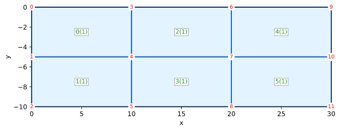
Solid Smith Figure 5.11 Qua4 Plane Strain Uy

Smith's Example 5.11 (Figure 5.11) on page 180

Smith IM, Griffiths DV, and Margetts L (2014) Programming the Finite Element Method, Wiley, Fifth Edition, 664p

Test goal

This test verifies a plane-strain simulation with prescribed displacements

Mesh

       Uy DISPLACEMENT
 0.0      0----------3----------6----------9
       Ux |          |          |          | Ux
       F  |          |          |          | F
       I  1----------4----------7---------10 I
       X  |          |          |          | X
       E  |          |          |          | E
-10.0  D  2----------5----------8---------11 D
         0.0       10.0       20.0       30.0
                    Ux and Uy FIXED

Mesh

Boundary conditions

Fix left edge horizontally
Fix right edge horizontally
Fix bottom edge horizontally and vertically
Displacement Uy = -1e-5 prescribed on top edge with x ≤ 10

Configuration and parameters

Static simulation
Young = 1e6
Poisson = 0.3
Plane-strain

Simulation and results

solid_smith_5d11_qua4_plane_strain_uy.rs

                                                  _   
timestep             t            Δt  iter    max(R)  
       1   1.000000e-1   1.000000e-1     .        .  
       .             .             .     1    2.21e1❋ 
       .             .             .     2  4.50e-16✅

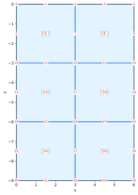
Solid Smith Figure 5.15 Qua8 Plane Strain

Smith's Example 5.15 (Figure 5.15) on page 183

Smith IM, Griffiths DV, and Margetts L (2014) Programming the Finite Element Method, Wiley, Fifth Edition, 664p

Test goal

This test verifies a plane-strain simulation with Qua8 elements and reduced integration.

Mesh

         1.0 kN/m²
        ↓↓↓↓↓↓↓↓↓↓↓
 0.0    0----1----2----3----4
        |         |         |
        5         6         7
        |         |         |
-3.0 Ux 8----9---10---11---12 Ux
     F  |         |         | F
     I 13        14        15 I
     X  |         |         | X
-6.0 E 16---17---18---19---20 E
     D  |         |         | D
       21        22        23
        |         |         |
-9.0   24---25---26---27---28
       0.0       3.0       6.0
           Ux and Uy FIXED

Mesh

Boundary conditions

Fix left edge horizontally
Fix right edge horizontally
Fix bottom edge horizontally and vertically
Distributed load Qn = -1 on top edge with x ≤ 3

Configuration and parameters

Static simulation
Young = 1e6
Poisson = 0.3
Plane-strain
NOTE: using reduced integration with 4 points

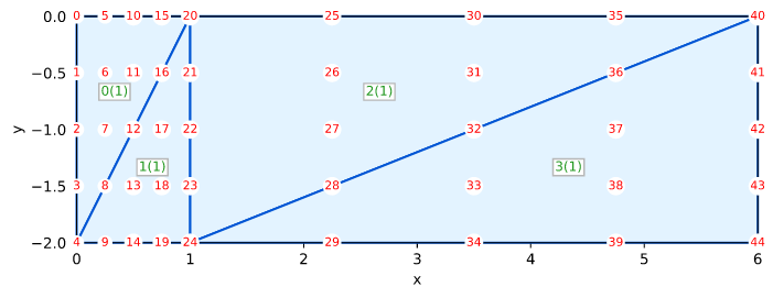
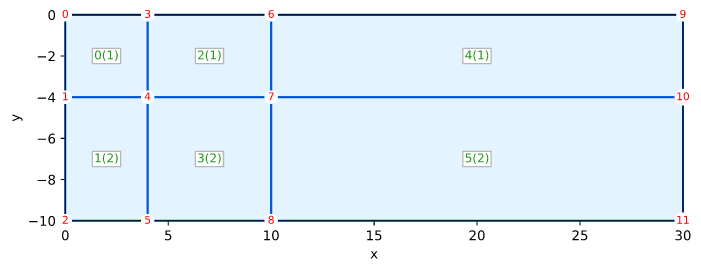
Solid Smith Figure 5.17 Qua4 Axisymmetric

Smith's Example 5.17 (Figure 5.17) on page 187

Smith IM, Griffiths DV, and Margetts L (2014) Programming the Finite Element Method, Wiley, Fifth Edition, 664p

Test goal

This test verifies an axisymmetric equilibrium problem.

Mesh

              1.0 kN/m²
         ↓↓↓↓↓↓↓↓↓↓↓↓↓↓↓↓↓↓↓
  0.0    0------3----------6-------------------9
      Ux | (0)  |   (2)    |        (4)        | Ux
      F  | [1]  |   [1]    |        [1]        | F
 -4.0 I  1------4----------7------------------10 I
      X  | (1)  |   (3)    |        (5)        | X
      E  | [2]  |   [2]    |        [2]        | E
-10.0 D  2------5----------8------------------11 D
        0.0    4.0       10.0                30.0
                     Ux and Uy FIXED

Mesh

Boundary conditions

Fix left edge horizontally
Fix right edge horizontally
Fix bottom edge horizontally and vertically
Concentrated load (Fy) on points 0, 3, 6, equal to
-2.6667, -23.3333, -24.0, respectively
Distributed load Qn = -1 on top edge with x ≤ 4

Configuration and parameters

Static simulation
Upper layer: Young = 100, Poisson = 0.3
Lower layer: Young = 1000, Poisson = 0.45
Plane-strain
NOTE: using 9 integration points

Simulation and results

solid_smith_5d15_qua8_plane_strain.rs

                                                  _   
timestep             t            Δt  iter    max(R)  
       1   1.000000e-1   1.000000e-1     .        .  
       .             .             .     1    2.00e0❋ 
       .             .             .     2  7.16e-15✅

Solid Smith Figure 5.24 Hex20 3D

Smith's Example 5.24 (Figure 5.24) on page 195

Smith IM, Griffiths DV, and Margetts L (2014) Programming the Finite Element Method, Wiley, Fifth Edition, 664p

Test goal

This test verifies a 3D simulation with Hex20.

Mesh

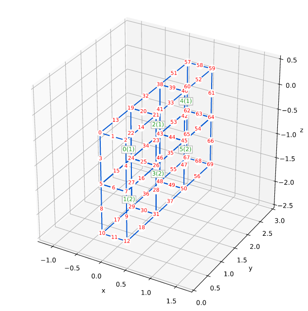
Boundary conditions

Horizontally fix the vertical boundary faces perpendicular to x on the "back side" with x=0
Horizontally fix the vertical boundary faces perpendicular to y on the "left side" with y=0
Set all Ux,Uy,Uz to zero for the horizontal boundary faces perpendicular to z on the "bottom" with z=0
Apply distributed load Qn = -1 on the portion of the top face with y ≤ 1
NOTE: The "front" and "right" faces with x>0 or y>0 are NOT fixed.

Configuration and parameters

Upper layer: Young = 100, Poisson = 0.3
Lower layer: Young = 50, Poisson = 0.3
Using reduced integration with 8 points

Simulation and results

solid_smith_5d24_hex20_3d.rs

                                                  _   
timestep             t            Δt  iter    max(R)  
       1   1.000000e-1   1.000000e-1     .        .  
       .             .             .     1   1.67e-1❋ 
       .             .             .     2  4.73e-16✅

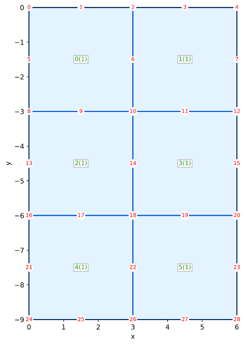
Solid Smith Figure 5.27 Qua9 Plane Strain

Smith's Example 5.27 (Figure 5.27) on page 200

Smith IM, Griffiths DV, and Margetts L (2014) Programming the Finite Element Method, Wiley, Fifth Edition, 664p

Test goal

This test verifies a plane-strain simulation with Qua9 elements and full integration. NOTE: This Example is similar to Example 5.15, with the difference being Qua9 elements.

Mesh

          1.0 kN/m²
         ↓↓↓↓↓↓↓↓↓↓↓
 0.0     0----1----2----3----4
         |         |         |
         5    6    7    8    9
         |         |         |
-3.0 Ux 10---11---12---13---14 Ux
     F   |         |         | F
     I  15   16   17   18   19 I
     X   |         |         | X
-6.0 E  20---21---22---23---24 E
     D   |         |         | D
        25   26   27   28   29
         |         |         |
-9.0    30---31---32---33---34
        0.0       3.0       6.0
            Ux and Uy FIXED

Mesh

Boundary conditions

Fix left edge horizontally
Fix right edge horizontally
Fix bottom edge horizontally and vertically
Distributed load Qn = -1 on top edge with x ≤ 3

Configuration and parameters

Static simulation
Young = 1e6
Poisson = 0.3
Plane-strain

Simulation and results

solid_smith_5d27_qua9_plane_strain.rs

                                                  _   
timestep             t            Δt  iter    max(R)  
       1   1.000000e-1   1.000000e-1     .        .  
       .             .             .     1    2.00e0❋ 
       .             .             .     2  5.66e-15✅

Solid Smith Figure 5.30 Tet4 3D

Smith's Example 5.30 (Figure 5.30) on page 202

Smith IM, Griffiths DV, and Margetts L (2014) Programming the Finite Element Method, Wiley, Fifth Edition, 664p

Test goal

This test verifies a 3D simulation with Tet4.

Mesh

Boundary conditions

Horizontally fix the vertical boundary faces perpendicular to x on the "back side" with x=0
Horizontally fix the vertical boundary faces perpendicular to y on the "left side" with y=0
Vertically fix the horizontal boundary faces perpendicular to z on the "bottom" with z=0
Apply vertical (Fz) concentrated loads to the top nodes:
Fz @ 0 and 5 = -0.1667, Fz @ 1 and 4 = -0.3333
(Do not USE more digits, as in the code, so we can compare with the Book results)

Configuration and parameters

Young = 100, Poisson = 0.3

Simulation and results

solid_smith_5d30_tet4_3d.rs

                                                  _   
timestep             t            Δt  iter    max(R)  
       1   1.000000e-1   1.000000e-1     .        .  
       .             .             .     1   3.33e-1❋ 
       .             .             .     2  9.30e-17✅

Dependencies

~17–30MB
~421K SLoC

3 releases (breaking)

Porous Media Simulator using the Finite Element Method

Contents

Introduction

Installation

Setting Cargo.toml

Examples

Heat: Arpaci Nonlinear 1d

Test goal

Mesh

Initial conditions

Boundary conditions

Configuration and parameters

Note

Simulation and results

Heat: Bhatti Example 1.5 Convection

Test goal

Mesh

Boundary conditions

Configuration and parameters

Simulation and results

Heat: Bhatti Example 6.22 Convection

Test goal

Mesh

Boundary conditions (see page 445)

Configuration and parameters

Simulation and results

Heat: Lewis Example 6.4.2 Transient 1d

Test goal

Mesh

Initial conditions

Boundary conditions

Configuration and parameters

Simulation and results

Heat: Mathematica Axisymmetric Nafems

Test goal

Initial conditions

Boundary conditions

Configuration and parameters

Simulation and results

Heat: Mathematica Axisymmetric Simple

Test goal

Mesh

Initial conditions

Boundary conditions

Configuration and parameters

Simulation and results

Rod: Bhatti Example 1.4 Truss

Test goal

Mesh

Boundary conditions

Configuration and parameters

Simulation and results

Solid Bhatti Example 1.6 Plane Stress

Test goal

Mesh

Boundary conditions

Configuration and parameters

Simulation and results

Solid Felippa Thick Cylinder Axisymmetric

Test goal

Mesh

Boundary conditions

Configuration and parameters

Simulation and results

Solid Smith Figure 5.2 Tri3 Plane Strain

Test goal

Mesh

Boundary conditions

Configuration and parameters

Simulation and results

Solid Smith Figure 5.7 Tri15 Plane Strain

Test goal

Boundary conditions

Configuration and parameters

Simulation and results

Solid Smith Figure 5.11 Qua4 Plane Strain Uy

Test goal

Mesh

Boundary conditions