4 releases
| 0.2.2 | Apr 20, 2023 |
|---|---|
| 0.2.1 | Apr 30, 2022 |
| 0.2.0 | Apr 27, 2022 |
| 0.1.0 | Feb 13, 2022 |
#457 in Simulation
440KB
6K
SLoC
fem_2d
A Rust library for 2D Finite Element Method computations, featuring:
- Highly flexible hp-Refinement
- Isotropic & Anisotropic h-refinements (with support for n-irregularity)
- Isotropic & Anisotropic p-refinements
- Generic shape function evaluation
- You can use one of the two built in sets of H(curl) conforming Shape Functions
- Or you can define your own by implementing the
ShapeFnTrait
- Two Eigensolvers
- Expressive Solution Evaluation
- Field solutions can easily be generated from an eigenvector
- Arbitrary functions of solutions can also be evaluated (ex: magnitude of a field)
- Solutions and expressions are easily printed to
.vtkfiles for plotting (using VISIT or similar tools)
Usage
Include this line in your Cargo.toml file under [dependencies]:
fem_2d = "0.1.0"
Please include one or more of the following citations in any academic or commercial work based on this repository:
- Corrado, Jeremiah; Harmon, Jake; Notaros, Branislav; Ilic, Milan M. (2022): FEM_2D: A Rust Package for 2D Finite Element Method Computations with Extensive Support for hp-refinement. TechRxiv. Preprint. https://doi.org/10.36227/techrxiv.19166339.v1
- Corrado, Jeremiah; Harmon, Jake; Notaros, Branislav (2021): A Refinement-by-Superposition Approach to Fully Anisotropic hp-Refinement for Improved Efficiency in CEM. TechRxiv. Preprint. https://doi.org/10.36227/techrxiv.16695163.v1
- Harmon, Jake; Corrado, Jeremiah; Notaros, Branislav (2021): A Refinement-by-Superposition hp-Method for H(curl)- and H(div)-Conforming Discretizations. TechRxiv. Preprint. https://doi.org/10.36227/techrxiv.14807895.v1
Documentation
The latest Documentation can be found here
Example
Solve the Maxwell Eigenvalue Problem on a standard Waveguide and print the Electric Fields to a VTK file.
This example encompasses most of the functionality of the library:
use fem_2d::prelude::*;

fn solve_basic_problem() -> Result<(), Box<dyn std::error::Error>> {
    // Load a standard air-filled waveguide mesh from a JSON file
    let mut mesh = Mesh::from_file("./test_input/test_mesh_a.json")?;

    // Set the polynomial expansion order to 4 in both directions on all Elems
    mesh.set_global_expansion_orders(Orders::new(4, 4));

    // Isotropically refine all Elems
    mesh.global_h_refinement(HRef::t());

    // Then anisotropically refine the resultant Elems in the center of the mesh
    let cenral_node_id = mesh.elems[0].nodes[3];
    mesh.h_refine_with_filter(|elem| {
        if elem.nodes.contains(&cenral_node_id) {
            Some(HRef::u())
        } else {
            None
        }
    });

    // Construct a Domain with H(curl) continuity conditions
    let domain = Domain::from_mesh(mesh, ContinuityCondition::HCurl);
    println!("Constructed Domain with {} DoFs", domain.dofs.len());

    // Construct a generalized eigenvalue problem for the Electric Field
    // (in parallel using the Rayon Global ThreadPool)
    let gep = galerkin_sample_gep_hcurl::<
        HierPoly,
        CurlCurl,
        L2Inner
    >(&domain, Some([8, 8]))?;

    // Solve the generalized eigenvalue problem using Nalgebra's Eigen-Decomposition
    // look for an eigenvalue close to 10.0
    let solution = nalgebra_solve_gep(gep, 10.0)?;
    println!("Found Eigenvalue: {:.15}", solution.value);

    // Construct a solution-field-space over the Domain with 64 samples on each "leaf" Elem
    let mut field_space = UniformFieldSpace::new(&domain, [8, 8]);

    // Compute the Electric Field in the X- and Y-directions (using the same ShapeFns as above)
    let e_field_names = field_space.xy_fields::<HierPoly>
        ("E", solution.normalized_eigenvector())?;

    // Compute the magnitude of the Electric Field
    field_space.expression_2arg(e_field_names, "E_mag", |ex, ey| {
        (ex.powi(2) + ey.powi(2)).sqrt()
    })?;

    // Print "E_x", "E_y" and "E_mag" to a VTK file
    field_space.print_all_to_vtk("./test_output/electric_field_solution.vtk")?;

    Ok(())
}
Mesh Refinement
A Mesh structure keeps track of the geometric layout of the finite elements (designated as Elems in the library), as well as the polynomial expansion orders on each element. These can be updated using h- and p-refinements respectively
h-Refinement:
h-Refinements* are implemented using the Refinement by Superposition (RBS) method
Technical details can be found in this paper: A Refinement-by-Superposition Approach to Fully Anisotropichp-Refinement for Improved Efficiency in CEM
Three types of h-refinement are supported:
- T: Elements are superimposed with 4 equally sized child elements
- U: Elements are superimposed with 2 child elements, such that the resolution is improved in the x-direction
- V: Elements are superimposed with 2 child elements, such that the resolution is improved in the y-direction
These are designated as an Enum: HRef, located in the h_refinements module. They can be executed by constructing a refinement as follows:
let h_iso = HRef::T;
let h_aniso_u = HRef::U(None);
let h_aniso_v = HRef::V(None);
...and applying it to an element or group of elements using one of the many h-refinement methods on Mesh.
Multi-step anisotropic h-refinements can be executed by constructing the U or V variant with Some(0) or Some(1). This will cause the 0th or 1st resultant child element to be anisotropically refined in the opposite direction.
Mesh coarsening is not currently supported
p-Refinement:
p-Refinements allow elements to support a range of expansion orders in the X and Y directions. These can be modified separately for greater control over resource usage and solution accuracy.
As a Domain is constructed from a Mesh, Basis Functions are constructed based on the elements expansion orders.
Expansion orders can be increased or decreased by constructing a PRef, located in the p_refinements module:
let uv_plus_2 = PRef::from(2, 2);
let u_plus_1_v_minus_3 = PRef::from(1, -3);
...and applying it to an element or group of elements using one of the many p-refinement methods on Mesh.
JSON Mesh Files
fem_2d uses .json files to import and export Mesh layouts.
- The input format is simplified and describes the geometry of the problem only.
- The output format describes the Mesh in it's refined state which is usefull for debugging and observing the refinement state.
Input Mesh Files
A Mesh can be constructed from a JSON file with the following format:
{
    "Elements": [
        {
            "materials": [eps_rel_re, eps_rel_im, mu_rel_re, mu_rel_im],
            "node_ids": [node_0_id, node_1_id, node_2_id, node_3_id],
        },
        {
            "materials": [1.0, 0.0, 1.0, 0.0],
            "node_ids": [1, 2, 4, 5],
        },
        {
            "materials": [1.2, 0.0, 0.9999, 0.0],
            "node_ids": [2, 3, 5, 6],
        }
    ],
    "Nodes": [
        [x_coordinate, y_coordinate],
        [0.0, 0.0],
        [1.0, 0.0],
        [2.0, 0.0],
        [0.0, 0.5],
        [1.0, 0.5],
        [2.0, 0.5],
    ]
}
(The first Element and Node are simply there to explain what variables mean. Those should not be included in an actual mesh file!)
The above file corresponds to this 2 Element mesh (with Node indices labeled):
    3               4               5
0.5 *---------------*---------------*
    |               |               |
    |      air      |    teflon     |
    |               |               |
0.0 *---------------*---------------*
 y  0               1               2
 x 0.0             1.0             2.0

Both Elements start with a polynomial expansion order of 1 upon construction.
This library does not yet support curvilinear elements. When that feature is added, this file format will also be extended to describe higher-order geometry.
Output Mesh Files
A refined Mesh can also be exported and visualized using this tool:
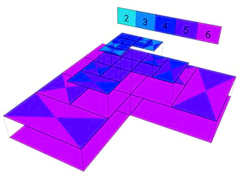
Solution Plotting
Solution figures like the ones below can be generated by exporting solutions as .vtk files and plotting using a compatible tool (such as Visit):


Community Guidelines / Code of Conduct
Contributions, questions, and bug-reports are welcome! Any pull requests, issues, etc. must adhere to Rust's Code of Conduct.
More details about how to contribute to this project can be found here.
Questions and bug-reports should be directed to the Issues tab.
Dependencies
~5MB
~97K SLoC