SCurve Motion Library

This library provides an S-curve motion profile computation framework with configurable jerk (acceleration ramp), acceleration, velocity, and distance constraints. It's designed to be both flexible and efficient, making it suitable for embedded systems, robotics, CNC controllers, and various motion control applications where smooth trajectory generation is required.

WARNING: The provided code may still contain errors and might not function correctly in some cases.

If you discover any errors, please let me know so that the code can be further improved.

Overview

An S-curve motion profile is a trajectory planning strategy that smoothly transitions acceleration (and hence velocity) over time. Instead of abrupt (piecewise-constant) acceleration, an S-curve incorporates jerk-limited ramps, significantly reducing mechanical stress, wear, and vibration.

Why Use an S-curve?

1. Reduced Vibration and Mechanical Stress
   By limiting jerk (the rate of change of acceleration), the system transitions between different velocity phases more smoothly. This helps prolong the lifetime of mechanical components, bearings, and motors because high accelerations are introduced gradually instead of instantaneously.

2. Better Control at High Speeds
   When moving at high velocities, abrupt changes in acceleration can cause instability or resonance. An S-curve approach prevents such instabilities.

3. Increased Precision
   Smooth trajectories enable more precise positioning, which is crucial in applications such as 3D printers, CNC routers, and robotic arms.

Key Features

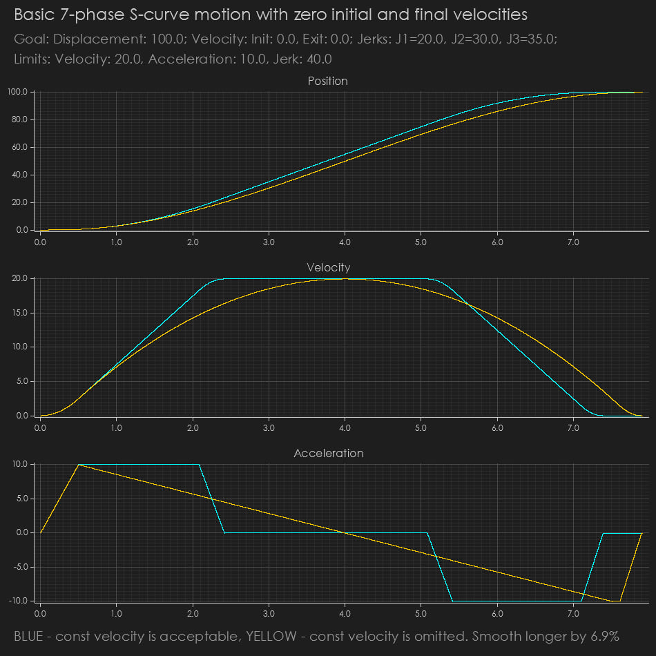
Exclude the Constant Velocity Phase

You can choose to not include a constant velocity phase (const_vel = false). Doing so may reduce vibrations and mechanical resonances if constant cruising is not needed (or if your travel distance is short). However, it may affect the overall travel time.

Individually Tunable Jerks

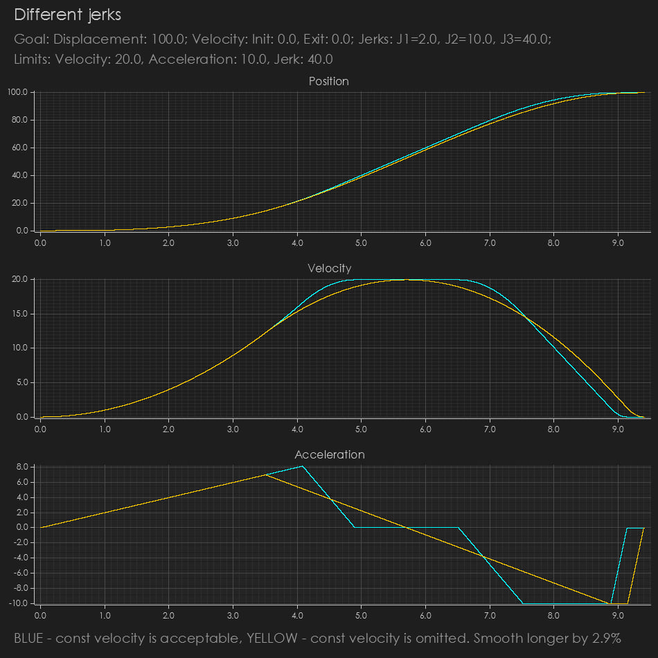
You can specify three jerk values:

• j_init for the initial velocity change,
• j_mid for cruising or smoothing around the maximum velocity phase,
• j_exit for the final velocity change.

This level of customization helps handle specific start/stop conditions separately from the mid-phase.

NOTE: When avoiding constant velocity, the algorithm may reduce j_mid.

WARNING: If positive motion is required and the delta velocity is impossible to achieve with the provided j_init and j_exit, these values will be proportionally scaled to fit within the target velocity delta and the required position change. However, they will be constrained by J_LIM.

Supports Infinite Values

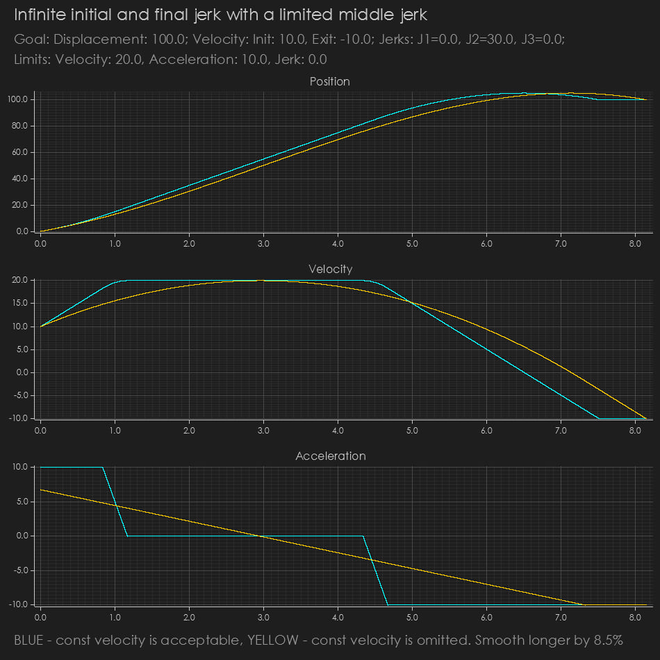
For certain combined profiles—like classical constant acceleration with minor jerk smoothing at high speeds—you can effectively set jerk to very large (“infinite”) or zero values to simulate an instant change. However, the jerk value will be constrained by J_LIM.

Similarly, for velocity and acceleration, if you don't care about the maximum velocity or acceleration, you can simply set them to f64::INFINITY or zero values. This will exclude the phases of constant acceleration or constant velocity.

NOTE: At least one of A_LIM or J_LIM should be a real limit. Otherwise, the mathematics will be unstable.

Works with Both Positive and Negative Velocities

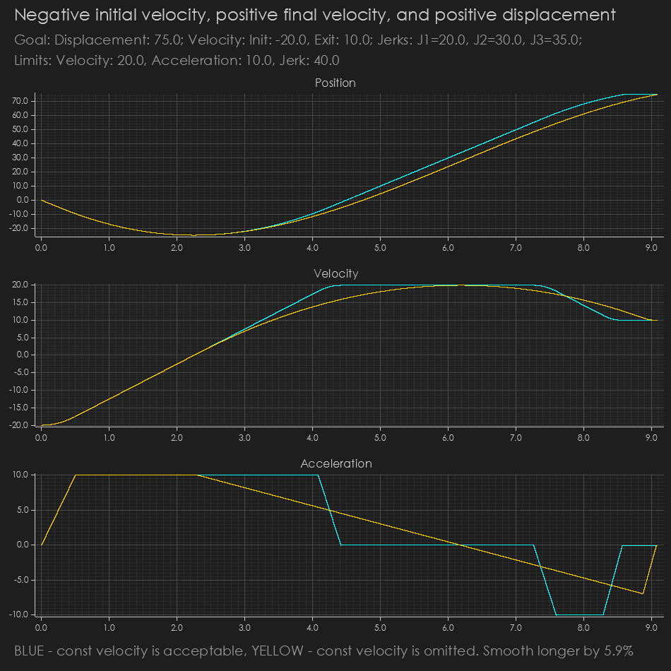
The code handles any sign of displacement (e.g., moving in reverse or forward) independently of the sign of the velocity. This means you can start or end at a negative velocity even if the distance to travel is positive. This feature may be useful in cases where a smooth and fast velocity change is required.

NOTE: Negative initial or exit velocity with positive displacement, or positive velocities with negative displacement, will cause position overshoot.

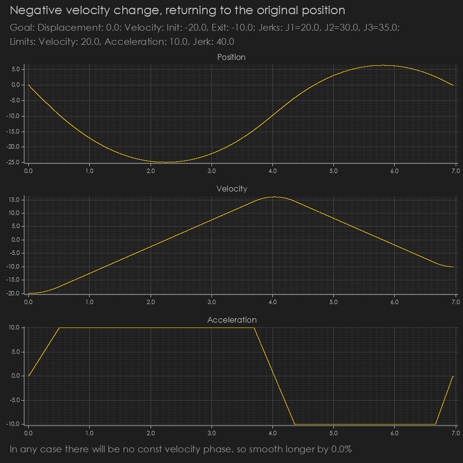
Support Zero Displacement if Initial and/or Exit Velocities Are Negative

Enables handling negative initial and final velocities even when the displacement is zero.

Configurable Limits

Velocity, acceleration, and jerk limits are easily set. This can help with hardware compliance or ensure you never exceed your motor/drive constraints.

Compute Coefficients Offline

The code is structured so you can perform all the heavy-lifting calculations (binary searches, polynomial fitting) ahead of time in a more powerful environment and then use the resulting coefficients in an embedded system. This separation of concerns is extremely helpful for real-time constraints on microcontrollers with limited resources.

Deep Dive into the Math

The core idea behind an S-curve is that jerk (the derivative of acceleration) remains limited to some maximum magnitude. Over each phase, acceleration changes linearly with time:

$$ \begin{aligned} \text{acc}(t) &= a_0 + j \cdot t,\ \text{vel}(t) &= \int \text{acc}(\tau), d\tau = v_0 + a_0 \cdot t + \frac{j \cdot t^2}{2},\ \text{pos}(t) &= \int \text{vel}(\tau), d\tau = s_0 + v_0 \cdot t + \frac{a_0 \cdot t^2}{2} + \frac{j \cdot t^3}{6} \end{aligned} $$

Within the code, we split the total motion into up to 7 phases (some phases may collapse if not required):

1. Acceleration ramp up from (v₀) (initial velocity)
2. Acceleration constant (if needed)
3. Acceleration ramp down to cruising velocity (v_lim)
4. Constant velocity (optional, can be skipped if const_vel = false)
5. Acceleration ramp up toward final velocity segment
6. Acceleration constant (if needed)
7. Acceleration ramp down to (v₁) (final velocity)

Velocity Change Calculations

To perform these calculations, the single function calc_dv_shift_t_s_a is mainly used.

• It computes the minimum time and distance needed for transitioning from v_init to v_exit, under a given jerk limit in the initial and exit phases, while respecting the a_limit
• The function breaks the velocity change into 3 phases:
  • Jerk from j_init (ramping acceleration up or down)
  • (Optional) constant acceleration if the peak acceleration hits acc_lim
  • Jerk from j_exit (ramping acceleration back down)

To do so, a few steps are needed:

1. Compute velocity difference = |v_init - v_exit|
2. Calculate the case when the acceleration limit is effectively not present (the case of absence of a constant acceleration phase) and estimate the time needed in the jerk-up phase T_J_INIT and jerk-down phase T_J_EXIT from the condition that total velocity change sums to velocity difference

$$ t_{j_{\text{init}}} = \sqrt{\frac{2 \cdot \Delta v \cdot j_{\text{exit}}}{j_{\text{init}} \cdot (j_{\text{init}} + j_{\text{exit}})}},~~~ t_{j_{\text{exit}}} = \sqrt{\frac{2 \cdot \Delta v \cdot j_{\text{init}}}{j_{\text{exit}} \cdot (j_{\text{init}} + j_{\text{exit}})}} $$

4. If the calculated peak acceleration exceeds acc_lim, the code clamps it to acc_lim and introduces a time t_a_const for the constant-acceleration phase.
5. Integrate polynomials to find exact position and velocity at each sub-phase.
6. Then calculate the total time, total distance, and final acceleration a_max used in the constant phase (if any).

This approach can be extended to handle sign changes (for negative velocities) by analyzing the sign of dV and applying the correct direction factor.

Binary Search for Fine-Tuning

For more complex scenarios — like reaching a middle velocity less than V_lim or adjusting the middle jerk J_mid — we employ binary searches (e.g., fit_j_mid, fit_v_max). We iteratively test candidate jerk or velocity values, compute the resulting distance/time, and compare it to the desired distance to converge on a solution within a given tolerance.

License

Copyright 2025 by Anton Khrustalev, CREAPUNK, http://creapunk.com

Licensed under the Apache License, Version 2.0 (the "License")