kalc

requires gnuplot for graphing, a modern terminal like windows terminal on windows

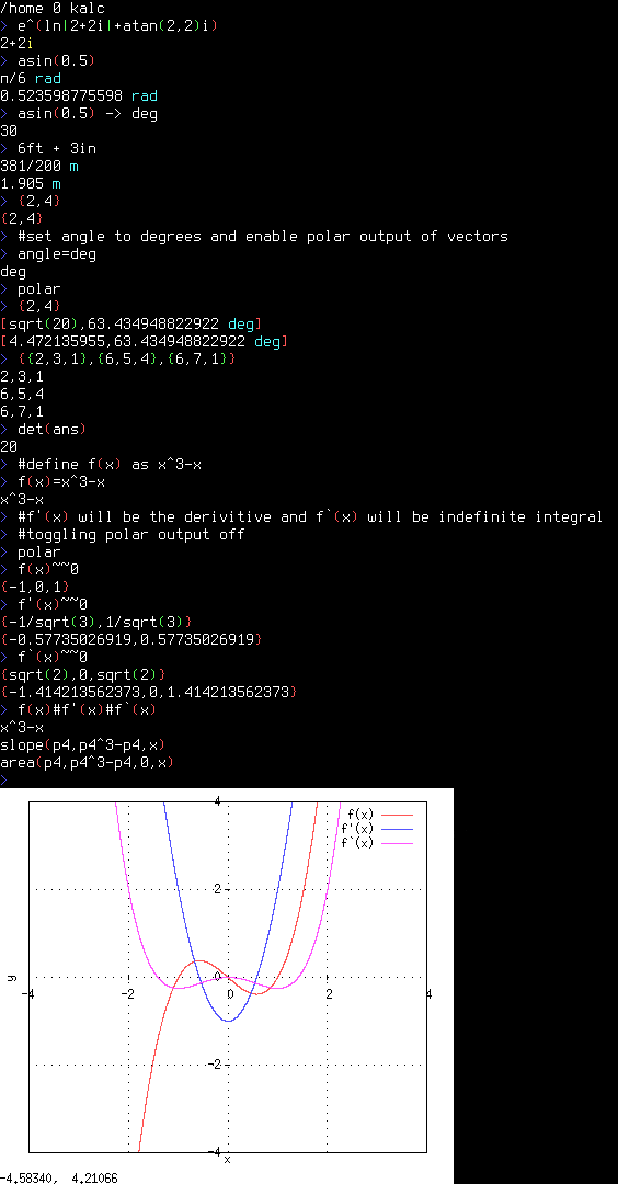
history file is stored in ~/.config/kalc.history

config file is stored in ~/.config/kalc.config

you can set permanent variables and functions in the file ~/.config/kalc.vars

parsing tries to comply with wolfram alpha

config defaults listed in kalc.config

issues

• 0's and infinities of trig functions don't show up as 0 or infinity.
• matrix to a fractional power is unsupported like {{2,3},{6,7}}^1.5
• loops(sum/prod etc) cant work with x,y,z as vars
• recursive formulas don't work
• inf + inf * i does not give inf+infi, infinitys generally dont well with complex numbers, like inf/i != -infi
• 1/0 != +-inf, digamma(-n) != +-inf, gamma(-n) != +-inf (and gamma subsidiarys)
• |2|x|| does not format as norm(2*norm(x)) it formats as norm(2)*x||, |ln|x|| works

build instructions

windows is not properly supported due to dependencys being weird, just use wsl

rust>=1.73.0 diffutils gcc m4 make

git clone https://github.com/bgkillas/kalc
cd kalc
cargo build --release
./target/release/kalc

usage

Usage: kalc [FLAGS] function_1 function_2 function_3...
FLAGS: --help (this message)
--tau fractions are shown in tau instead of pi
--deg compute in degrees
--rad compute in radians
--grad compute in gradians
--2d=[num] number of points to graph in 2D
--3d=[x],[y] number of points to graph in 3D
--xr=[min],[max] x range for graphing
--yr=[min],[max] y range for graphing
--zr=[min],[max] z range for graphing
--range=[num] sets all ranges to [-num],[num]
--point [char] point style for graphing
--sci toggles scientific notation
--base=[num] sets the number base (2,8,16)
--prompt toggles the prompt
--color toggles color
--comma toggles comma seperation
--vars toggles default variables
--line toggles line graphing
--rt toggles real time printing
--polar toggles displaying polar vectors
--frac toggles fraction display
--frac_iter=[num] how many iterations to check for fractions
--prec=[num] sets the precision
--deci=[num] sets how many decimals to display, -1 for length of terminal, -2 for maximum decimal places, may need to up precision for more decimals
--def ignores config file
--multi toggles multi line display for matrixes
--tabbed toggles tabbed display for matrixes
--debug displays computation time in nanoseconds
--depth display 2d complex graphs in 3d with imag #'s going up/down on the z axis
--small_e use small e notation, like 5e2=5*10^2, instead of capital 'E' for scientific notation. only works with a number before and number or '-' sign after the 'e' otherwise assumes euler number

- flags can be executed in runtime just without the dashes
- Type "colors=" to see color settings
- Type "exit" to exit the program
- Type "clear" to clear the screen
- Type "history [arg]" to see the history, arg indexes it if specified
- Type "vars" to list all variables
- Type "lvars" to list all variables without equating them
- Type "_" to use the previous answer
- Type "a={expr}" to define a variable
- Type "f(x)=..." to define a function
- Type "f(x,y,z...)=..." to define a multi variable function
- Type "...=" display parsed input, show values of stuff like xr/deci/prec etc
- Type "f...=null" to delete a function or variable
- Type "{x,y,z...}" to define a cartesian vector
- Type "[radius,theta,phi]" to define a polar vector (same as car{vec})
- Type "{vec}#" to graph a vector
- Type "{mat}#" to graph a matrix
- Type "number#" to graph a complex number
- Type "{{a,b,c},{d,e,f},{g,h,i}}" to define a 3x3 matrix
- Type "rnd" to generate a random number

Operators:
- +, -, *, /, //, ^, ^^, %, <, >, <=, >=, |x|, ±/+-
- !x (subfact), x! (fact), x!! (doublefact)
- && (and), || (or), == (equals), != (not equals)
- >> (right shift), << (left shift)

Trigonometric functions:
- sin, cos, tan, asin, acos, atan, atan(x,y)
- csc, sec, cot, acsc, asec, acot
- sinh, cosh, tanh, asinh, acosh, atanh
- csch, sech, coth, acsch, asech, acoth

Other functions:
- sqrt, cbrt, square, cube, quad(a,b,c)(quadratic formula)
- ln, log(base,num), root(base,exp), sum(var,func,start,end), prod(var,func,start,end)
- abs, sgn, arg
- ceil, floor, round, int, frac
- fact(real), doublefact(real), subfact(natural)
- sinc, cis, exp
- zeta, gamma, erf, erfc, digamma, ai, binomial/bi/C, P(n,r) (all real only)
- deg, rad, grad (all real only)
- re, im, split(x+yi={x,y})
- factors, prime
- slog(a,b)
- vec(var,func,start,end) mat(var,func,start,end) (makes a vector/matrix) start..end is a shortcut to vec(n,n,start,end)

Vector functions:
- dot({vec1},{vec2}), cross({vec1},{vec2}), proj/project({vec1},{vec2})
- angle({vec1},{vec2})
- norm, normalize
- abs, len, any, all
- max, min, mean, median, mode, sort
- reverse, link
- part({vec},col), sum, prod
- pol{vec} outputs (radius, theta, phi)
- car{vec} outputs (x, y, z)
- other functions are applied like sqrt{2,4}={sqrt(2),sqrt(4)}

Matrix functions:
- trace/tr, determinant/det, inverse/inv
- transpose/trans, adjugate/adj, cofactor/cof, minor
- part({mat},col,row), flatten, sum, prod
- abs, norm
- len, wid
- max, min, mean, mode
- I(n) produces n identity matrix
- rotate(theta) produces a rotational matrix
- other functions are applied like sqrt{{2,4},{5,6}}={{sqrt(2),sqrt(4)},{sqrt(5),sqrt(6)}} 

Constants:
- c: speed of light, 299792458 m/s
- g: gravity, 9.80665 m/s^2
- G: gravitational constant, 6.67430E-11 m^3/(kg*s^2)
- h: planck's constant, 6.62607015E-34 J*s
- ec: elementary charge/electron volt, 1.602176634E-19 C/J
- me: electron mass, 9.1093837015E-31 kg
- mp: proton mass, 1.67262192369E-27 kg
- mn: neutron mass, 1.67492749804E-27 kg
- k: coulomb's constant, 8.9875517923E9 N*m^2/C^2
- Na: avogadro's number, 6.02214076E23 1/mol
- R: gas constant, 8.31446261815324 J/(mol*K)
- kB: boltzmann constant, 1.380649E-23 J/K
- phi/φ: golden ratio, 1.6180339887~
- e: euler's number, 2.7182818284~
- pi/π: pi, 3.1415926535~
- tau/τ: tau, 6.2831853071~

Digraph:
hit escape then a letter
a=>α, A=>Α, b=>β, B=>Β, c=>ξ, C=>Ξ, d=>Δ, D=>δ,
e=>ε, E=>Ε, f=>φ, F=>Φ, g=>γ, G=>Γ, h=>η, H=>Η,
i=>ι, I=>Ι, k=>κ, Κ=>Κ, l=>λ, L=>Λ, m=>μ, M=>Μ,
n=>ν, Ν=>Ν, o=>ο, O=>Ο, p=>π, P=>Π, q=>θ, Q=>Θ,
r=>ρ, R=>Ρ, s=>σ, S=>Σ, t=>τ, T=>Τ, u=>υ, U=>Υ,
w=>ω, W=>Ω, y=>ψ, Y=>Ψ, x=>χ, X=>Χ, z=>ζ, Z=>Ζ,
==>±, `=>ⁱ _=>∞
numbers/minus sign convert to superscript acting as exponents

example usage

kalc
> 1+1
2
> f(x)=sin(2x)
> f(x) // graphs f(x) in 2D
> f(pi/2) // evaluates f(x) at x=pi/2, so sin(2pi/2)=sin(pi)=0
0
> f(x,y)=x^2+y^2
> f(1,2) // evaluates f(x,y) at x=1, y=2, so 1^2+2^2=5
5
> f(x,y) // graphs f(x,y) in 3D
> a=3^3
> cbrt(a)
3
> im(exp(xi)) // graphs the imag part of exp(xi) in 2D, so sin(x)
> f(x,y,z,w)=x+y+z+w
> f(1,2,3,4) // evaluates f(x,y,z,w) at x=1, y=2, z=3, w=4, so 1+2+3+4=10
10
> f(x,y,2,5) // graphs f(x,y,2,5) in 3D with z=2 and w=5 so x+y+2+5
> f(x,y,2,5)= // displays how its parsed
((x)+(y)+(2)+(5))
> f(2,5,x,y) // graphs f(2,5,x,y) in 3D with x=2 and y=5 so 2+5+x+y, to graph x and y have to be the unknown variables
> |z| // graphs |(x+yi)| in 3D
> deg // enables degrees
> pol({5,3,2}+{1,2,3}) // prints {magnitude, theta, phi} of {5,3,2}+{1,2,3}
{9.273618495496,57.373262293469,39.805571092265}

echo -ne 'sqrt(pi) \n pi^2'|kalc
1.7724538509055159
9.869604401089358

kalc 'sqrt(pi)' 'pi^2'
1.7724538509055159
9.869604401089358

echo -ne 'sin(x)#cos(x)'|kalc // graphs sin(x) and cos(x) in 2D
kalc 'sin(x)#cos(x)' // graphs sin(x) and cos(x) in 2D

graphing

chars available for point style:
. - dot
+ - plus
x - cross
* - star
s - empty square
S - filled square
o - empty circle
O - filled circle
t - empty triangle
T - filled triangle
d - empty del (upside down triangle)
D - filled del (upside down triangle)
r - empty rhombus
R - filled rhombus