47 releases
| 0.4.8 | May 9, 2024 |
|---|---|
| 0.4.6 | Mar 23, 2024 |
| 0.4.5 | Dec 17, 2023 |
| 0.4.2 | Oct 20, 2023 |
| 0.1.5 | Jul 31, 2022 |
#32 in Machine learning
1,057 downloads per month
745KB
5.5K
SLoC

Forust
A lightweight gradient boosting package
Forust, is a lightweight package for building gradient boosted decision tree ensembles. All of the algorithm code is written in Rust, with a python wrapper. The rust package can be used directly, however, most examples shown here will be for the python wrapper. For a self contained rust example, see here. It implements the same algorithm as the XGBoost package, and in many cases will give nearly identical results.
I developed this package for a few reasons, mainly to better understand the XGBoost algorithm, additionally to have a fun project to work on in rust, and because I wanted to be able to experiment with adding new features to the algorithm in a smaller simpler codebase.
All of the rust code for the package can be found in the src directory, while all of the python wrapper code is in the py-forust directory.
Documentation
Documentation for the python API can be found here.
Installation
The package can be installed directly from pypi.
pip install forust
To use in a rust project add the following to your Cargo.toml file.
forust-ml = "0.4.8"
Usage
For details on all of the methods and their respective parameters, see the python api documentation.
The GradientBooster class is currently the only public facing class in the package, and can be used to train gradient boosted decision tree ensembles with multiple objective functions.
Training and Predicting
Once, the booster has been initialized, it can be fit on a provided dataset, and performance field. After fitting, the model can be used to predict on a dataset. In the case of this example, the predictions are the log odds of a given record being 1.
# Small example dataset
from seaborn import load_dataset

df = load_dataset("titanic")
X = df.select_dtypes("number").drop(columns=["survived"])
y = df["survived"]

# Initialize a booster with defaults.
from forust import GradientBooster
model = GradientBooster(objective_type="LogLoss")
model.fit(X, y)

# Predict on data
model.predict(X.head())
# array([-1.94919663,  2.25863229,  0.32963671,  2.48732194, -3.00371813])

# predict contributions
model.predict_contributions(X.head())
# array([[-0.63014213,  0.33880048, -0.16520798, -0.07798772, -0.85083578,
#        -1.07720813],
#       [ 1.05406709,  0.08825999,  0.21662544, -0.12083538,  0.35209258,
#        -1.07720813],
When predicting with the data, the maximum iteration that will be used when predicting can be set using the set_prediction_iteration method. If early_stopping_rounds has been set, this will default to the best iteration, otherwise all of the trees will be used.
If early stopping was used, the evaluation history can be retrieved with the get_evaluation_history method.
model = GradientBooster(objective_type="LogLoss")
model.fit(X, y, evaluation_data=[(X, y)])

model.get_evaluation_history()[0:3]

# array([[588.9158873 ],
#        [532.01055803],
#        [496.76933646]])
Inspecting the Model
Once the booster has been fit, each individual tree structure can be retrieved in text form, using the text_dump method. This method returns a list, the same length as the number of trees in the model.
model.text_dump()[0]
# 0:[0 < 3] yes=1,no=2,missing=2,gain=91.50833,cover=209.388307
#       1:[4 < 13.7917] yes=3,no=4,missing=4,gain=28.185467,cover=94.00148
#             3:[1 < 18] yes=7,no=8,missing=8,gain=1.4576768,cover=22.090348
#                   7:[1 < 17] yes=15,no=16,missing=16,gain=0.691266,cover=0.705011
#                         15:leaf=-0.15120,cover=0.23500
#                         16:leaf=0.154097,cover=0.470007
The json_dump method performs the same action, but returns the model as a json representation rather than a text string.
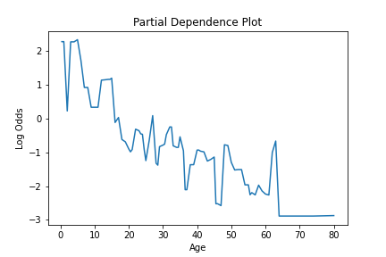
To see an estimate for how a given feature is used in the model, the partial_dependence method is provided. This method calculates the partial dependence values of a feature. For each unique value of the feature, this gives the estimate of the predicted value for that feature, with the effects of all features averaged out. This information gives an estimate of how a given feature impacts the model.
This information can be plotted to visualize how a feature is used in the model, like so.
from seaborn import lineplot
import matplotlib.pyplot as plt

pd_values = model.partial_dependence(X=X, feature="age", samples=None)

fig = lineplot(x=pd_values[:,0], y=pd_values[:,1],)
plt.title("Partial Dependence Plot")
plt.xlabel("Age")
plt.ylabel("Log Odds")

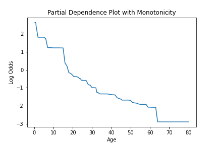
We can see how this is impacted if a model is created, where a specific constraint is applied to the feature using the monotone_constraint parameter.
model = GradientBooster(
    objective_type="LogLoss",
    monotone_constraints={"age": -1},
)
model.fit(X, y)

pd_values = model.partial_dependence(X=X, feature="age")
fig = lineplot(
    x=pd_values[:, 0],
    y=pd_values[:, 1],
)
plt.title("Partial Dependence Plot with Monotonicity")
plt.xlabel("Age")
plt.ylabel("Log Odds")

Feature importance values can be calculated with the calculate_feature_importance method. This function will return a dictionary of the features and their importances. It should be noted that if a feature was never used for splitting it will not be returned in importance dictionary. This function takes the following arguments.
model.calculate_feature_importance("Gain")
# {
#   'parch': 0.0713072270154953,
#   'age': 0.11609109491109848,
#   'sibsp': 0.1486879289150238,
#   'fare': 0.14309120178222656,
#   'pclass': 0.5208225250244141
# }
Saving the model
To save and subsequently load a trained booster, the save_booster and load_booster methods can be used. Each accepts a path, which is used to write the model to. The model is saved and loaded as a json object.
trained_model.save_booster("model_path.json")

# To load a model from a json path.
loaded_model = GradientBooster.load_booster("model_path.json")
Dependencies
~2–3MB
~65K SLoC