2 unstable releases
| 0.3.0 | Dec 28, 2021 |
|---|---|
| 0.1.0 | Aug 6, 2021 |
#292 in Geospatial
125KB
250 lines
![]()
zonebuilder
A rust crate for building zones.
It is an in-progress project to implement the functionality in the
zonebuilder R package
in the systems programming language Rust.
Why?
- It should eventually enable more people to benefit from free and open source software for creating zoning systems because Rust enables the creation of binaries for Windows, Mac and the free and open source Linux operating system on which the package was originally developed
- To enable deployment of the zonebuilder techniques online, as demonstrated in the web folder (Rust can also compile to WASM enabling complex applications such as A/B Street to run in browser — the thinking being if that can run in browser surely as simple application to build zones can!)
- Computational efficiency: the process of building zones is not
particularly computationally intensive but this Rust crate may
eventually be fast and quick to install and use, possibly from
higher level languages such as R using Rust interfaces such as
extendr - For fun and education: as a simple crate it serves as a good way to show how Rust code is organised and how it works
Installation of the Rust crate
To install the zonebuilder crate, you need first install
Rust.
Install the latest version on crates.io with
cargo install zonebuilder
You can install the development version as follows:
cargo install --git https://github.com/zonebuilders/zonebuilder-rust --branch main
Download and run binaries
Rust can create binaries for all major operating systems. Watch this space for how to run zonebuilders using a binary (no compilation or Rust toolchain required).
Running zonebuilder from the system command line
The zonebuilder binary has a command line interface. Assuming you are
installing the crate locally, you can build the binary for Windows, Mac
and Linux system shells as follows:
cargo build
## Finished dev [unoptimized + debuginfo] target(s) in 0.02s
You can see instructions on using the tool with the following command:
./target/debug/zonebuilder -h
## zb 0.1.0
## Configures a clockboard diagram
##
## USAGE:
##     zonebuilder [FLAGS] [OPTIONS]
##
## FLAGS:
##     -h, --help         Prints help information
##         --projected    Is the data projected?
##     -V, --version      Prints version information
##
## OPTIONS:
##     -d, --distances <distances>...
##             The distances between concentric rings. `triangular_sequence` is useful to generate these distances
##             [default: 1.0,3.0,6.0,10.0,15.0]
##     -s, --num-segments <num-segments>
##             The number of radial segments. Defaults to 12, like the hours on a clock [default: 12]
##
##     -v, --num-vertices-arc <num-vertices-arc>
##             The number of vertices per arc. Higher values approximate a circle more accurately [default: 10]
##
##     -p, --precision <precision>
##             The number of decimal places in the resulting output GeoJSON files. Set to 6 by default. Larger numbers mean
##             more precision, but larger file sizes [default: 6]
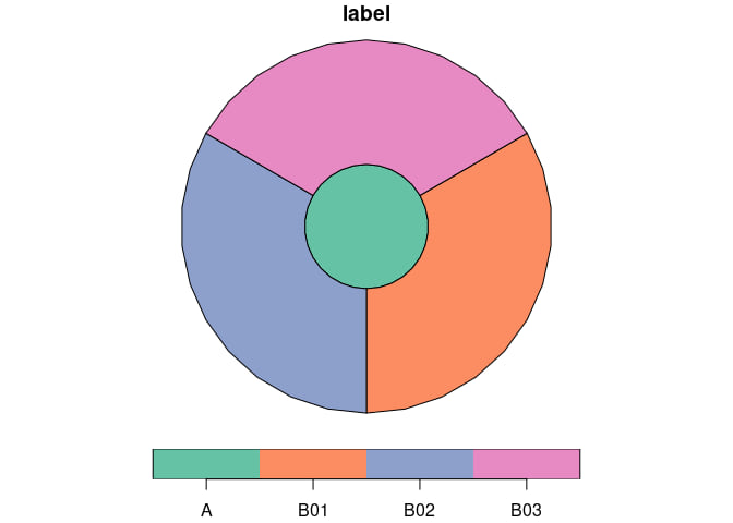
Let’s try making zones with fewer segments and circles (specified by the
-s and -d arguments respectively):
./target/debug/zonebuilder -s 3 -d 1.0,3.0 > zones.geojson
The The result looks like this:
You can also set the precision of outputs. The default is 6 decimal places, as shown in the output below:
head(sf::st_coordinates(z))
##             X        Y L1 L2
## [1,] 0.000000 0.009043  1  1
## [2,] 0.001867 0.008846  1  1
## [3,] 0.003653 0.008261  1  1
## [4,] 0.005280 0.007316  1  1
## [5,] 0.006675 0.006051  1  1
## [6,] 0.007779 0.004521  1  1
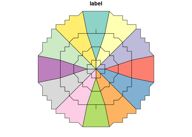
Let’s see the output when a precision of 2 decimal places is used:
./target/debug/zonebuilder --precision 2 > zones.geojson
That results in this:
You can run the crate as follows (note the use of -- to pass the
arguments to the zonebuilder binary not cargo run):
cargo run -- --precision 3 > zones.geojson
##     Finished dev [unoptimized + debuginfo] target(s) in 0.02s
##      Running `target/debug/zonebuilder --precision 3`
Take a look at the output:
head -n 20 zones.geojson
## {
##   "features": [
##     {
##       "geometry": {
##         "coordinates": [
##           [
##             [
##               0.0,
##               0.009
##             ],
##             [
##               0.0,
##               0.009
##             ],
##             [
##               0.0,
##               0.008
##             ],
##             [
##               0.001,
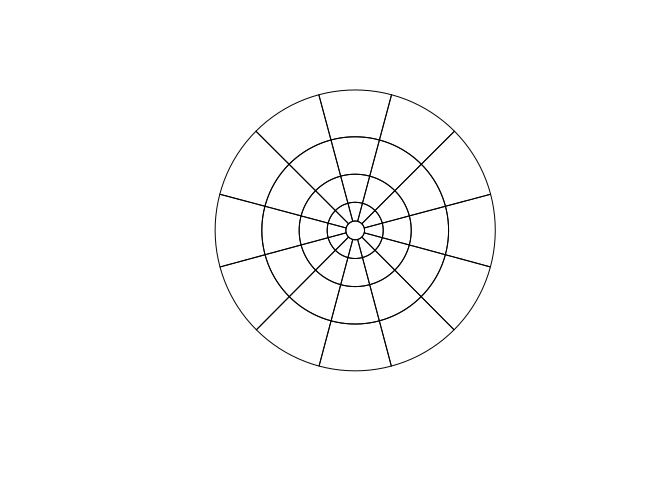
Then read in the GeoJSON file with another tool, e.g. R (this step runs
from an R console that has the sf library installed):
zones = sf::read_sf("zones.geojson")
plot(zones)
# interactive version:
# mapview::mapview(zones)
file.remove("zones.geojson")
## [1] TRUE
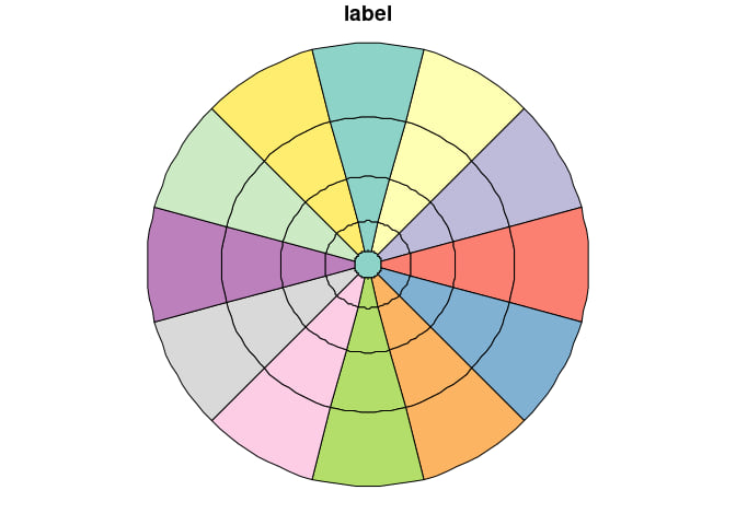
You can generate the same plot in R with the zonebuilder package as
follows:
zones = zonebuilder::zb_zone(x = "london", n_circles = 5)
## Loading required namespace: tmaptools
plot(zones$geometry)
Dependencies
~8.5MB
~155K SLoC