load_lpp (log - process - plot) 🦀

This crate compiles the following three binaries for logging, preprocessing, and plotting load time series. The application is written in Rust and targets low-level optimization and long-term stability.

1 load_log_dad141

CLI application to log load cells via the common DAD 141.1 digital amplifier with TCP-UTF8. The application allows automatic logging at rounded intervals of minutes or hours that are divisors of 1 day. Valid minutes intervals are 1, 2, 3, 5, 10, 15, 20, 30, and 60 minute(s). Valid hours intervals are 1, 2, 3, 6, 12, and 24 hour(s). The standard format RFC 3339 - ISO 8601 is used for the datetime to be more general and robust to time zones and daylight saving.

2 load_process

This CLI application processes the load time series with the following steps:

1. Read and parse the logged load time series.
2. Convert all datetime to a chosen time zone, i.e., removing daylight saving if needed or changing the time zone is desired.
3. Make the time series continuous using the minimum time interval found in the data.
4. Optionally, replace logging errors with NAN.
5. Optionally, replace given datetimes from an input file with NAN (e.g., values disturbed by maintenance).
6. Optionally, replace a given daily interval with NAN (e.g., daily temperature effects or maintenance period).
7. Optionally, automatically detect and report anomalous periods that would be hardly smoothed and corrected by the following moving average.
8. Optionally, use a weighted moving average to smooth the time series (e.g., wind and temperature) and fill the NAN values. It uses a moving average with linear weights between a user-defined central weight (typically the max weight) and a side weight (typically the minimum weight). The width of the window can be adjusted by specifying the number of data points on each side, this parameterization guaranties the window symmetry. Constraints can be set to define when the missing information is too large to fill the NAN values (maximum number of missing load values or their cumulative associated weight).
9. The CLI application saves a new csv file compatible with load_plot.

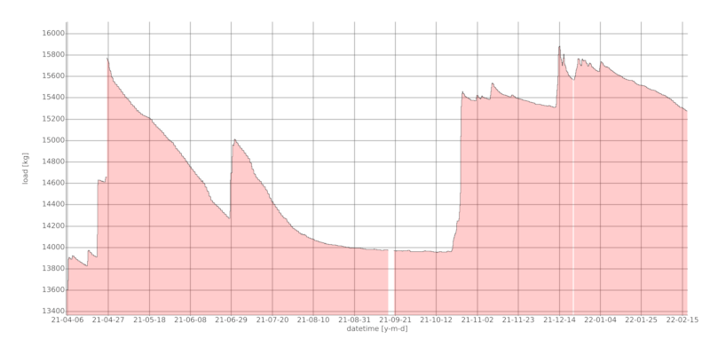
3 load_plot

CLI application to plot the load time series saved by dad141_log or load_process. The application automatically adjust the datetime format. The output format of the figure is svg.

Note, throughout the crate, load is used for the load cells data, while weight is used for the moving average.

Documentation: rust_crate

The CLI applications are written in the Rust programming language.

Addition Notes

DAD141.1

General

• Remove the seal switch jumper to enable all the commands, that is just for legal applications.
• Use function 2.4 to display the actual raw voltage mV/V.
• Menu 3.1 for overload, make sure it is above the required maximum load.

Calibration: Zero (intercept) and Span (slope, span calibration)

See examples in the DAD manual and section 7.4 (pag. 34) in the DOP manual.

• Zeroing with function 1.2 - CZ (gravimetric) or 1.3 - AZ (electronic), this associates the current measured voltage (mV/V) with the zero reading.
• Set span_kg with function 2.1, set RO_kg_sum.
• Set span_V, from the formula below, with function 2.3.

Calculate the span value (span_V)

span_kg = RO_kg_sum = RO_kg_1 + RO_kg_2 + ... RO_kg_n.

For example, span_kg = 20kN * 6 load cells = 120 kN = 120 = 12,236.5921 kg. Set RO_kg_sum in DAD 141.1 function 2.1.

RO_V_1 + RO_V_2 + ... + RO_V_n = RO_V_sum, in mV/V.

span_V = (V_sum / kg_sum) * kg_max, in mV/V. In our case 12.00062 / 6 = 2.000103333 mV/V.

In our case, SPAN_V = 2.00032 + 2.00034 + 1.99979 + 2.00014 + 2.00011 + 1.99992 = 12.00062 mV/V. Put span_V in function 2.3.

Where:

• RO_V is the voltage output (mV/V) at the rated output (RO) from the calibration certificates.
• RO_kg is the rated output, always from calibration.

kg from mV

kg@x = (mV@x / (mV@RO * ExcitationVoltage)) * kg@RO

For example, if kg@RO = 2039.43 kg mv/V@RO ~ 2 mv/V ExcitationVoltage should be 5 V

2040 kg should give 10mV (i.e., 2 mv/V * 5 V) 1020 kg should give 5mV (i.e., 2 mv/V * 5 V / 2) in general, 204 kg = 1 mV

Format

The application expects the 10-byte DAD format, with flexibility on the position of the decimal separator. The first two characters are the description of the value and are excluded from the parsing of the numerical load value. However, the raw string is also written into the csv file to avoid losing information on the type of reading and recover the values in case of parsing errors. Possible whitespace-property characters (Unicode standard) will be correctly trimmed and ignored.

Installation of the load cells and mounting modules

Mounting modules

Three types of mounting modules are used to obtain the correct degrees of freedom, matching the deformation of the system.

1. Fixed: No mobility, the modules fixes the system point in that position (0D freedom).
2. Bumper: Constrains the movement in one direction (1D freedom).
3. Free: It allows the movement in all the directions, within the load cell plane (2D freedom).

Alignment

Align the load cells considering the degrees of freedom of the mechanical deformation. In particular, pay attention to the fixed and bumper load cell, and their alignment with respect to the main deformation at the bumper. See figures are in the manuals.

Lubricant/Grease

It is used to protect the mobile parts of the mounting module during their movement (rocker pin and matching top surface). Some examples are:

• Mettler Toledo manual, Loctite Anti Seize, Food Grade
• Flintec, At Flintec use RENOLIT ST-80, by Fuchs. However, they provided a similar one already with the load cells.

Remote/SSH logging

The command line applications are suited for remote monitoring. A possible solution to establish remote and persistent connection is the use of ssh and tmux. In addition, scp can be used to copy-transfer the data.

Find ip and/or hostname

1. find the ip address, e.g., ifconfig.
2. find the hostname with host ipaddr_from_ifconfig.

Starting

1. ssh to raspberry pi, ssh user@ip
2. open tmux, tmux
3. start the logging process, see ./compiled_binary --help
4. detach the tmux session n from terminal with Ctrl+b then d, which returns [detached (from session n)]
5. check if tmux session is still there with tmux ls, it should return n: 1 windows (created datetime 2), where datetime is of point 2
6. close terminal/ssh connection, exit, it returns Connection to uset@ip closed

Check logging

1. ssh to raspberry pi, ssh user@ip, as step 1 of starting
2. find tmux session with tmux ls, as step 5 of starting
3. attach the session with tmux attach -t n, where n is the number from starting step 4
4. repeat steps 4, 5, 6 from starting

Copy the data

1. open terminal and copy file from raspberry to laptop with scp, e.g., scp user@localhost:~/path/to/file/loadcells.csv ./Desktop/

Close logging

1. ssh to raspberry pi, ssh user@ip, as step 1 of starting
2. find tmux session with tmux ls, as step 5 of starting
3. close running logging with Ctrl+c, should return [exited]
4. double check with tmux ls, should return no server running on ...

Additional details on remote connections

• How to recover a shell after a disconnection
• How to keep processes running after ending ssh session?
• TcpStream write silently loses one message