13 releases (1 stable)
| 1.0.0 | Mar 27, 2022 |
|---|---|
| 0.9.0 | Jan 22, 2022 |
| 0.8.4 | Jan 22, 2022 |
| 0.7.0 | Jan 1, 2022 |
| 0.4.2 | Oct 12, 2021 |
#1051 in Algorithms
131 downloads per month
135KB
1.5K
SLoC
![]()
![]()
![]()
![]()
Shout out: I want to say thanks to Red Blob Games, they have a fantasic set of guides/tutorials detailing hexagonal spaces and the associated geometries which have helped me enourmously in Rust-ifying concepts
hexagonal_pathfinding_astar
This library is an implementation of the A-Star pathfinding algorithm tailored for traversing a bespoke collection of weighted hexagons. It's intended to calculate the most optimal path to a target hexagon where you are traversing from the centre of one hexagon to the next along a line orthogonal to a hexagon edge. The algorithm has been implemented for Offset, Axial and Cubic coordinate systems with a selection of helper functions which can be used to convert between coordinate systems, calculate distances between hexagons and more.
It's rather different in that it follows a convention whereby a hexagon has a measurement which reflects the difficulty of traversing a distance over time called complexity (don't ask why I didn't name it velocity).
E.g
    ___________
   /     ^     \
  /      |      \
 /    c  |       \
 \       |       /
  \      ▼      /
   \___________/
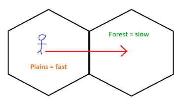
For a grid of perfectly flush hexagons the distance from the centre to the midpoint of an edge is the same in all directions. This library is akin to idea that you wake up in a 'hexagon world' and you can only move from the centre of one hexagon to another in a straight line, but while distance is static you'll find that as you cross the boundary of one hexagon into another you'll suddenly be sprinting instead of slow-motion walking.
Generic example: Imagine leaving your house and standing by the side of a road. You want to go to a shop and there's two to choose from, one to the left and one to the right. They are both 100 meters away from you however if you go left you'll have to walk through a busy high street whereas going right leads to a much quieter area of town where you can ride a bicycle. To complete your shopping as quickly as possible you'll want to go right. This is what I mean by complexity, it isn't a measure of a hexagons width, all distances are the same, rather it is a measure of how quickly you can traverse it.
Another example, say you're a character in an RPG standing on a hexagon which denotes an open space. If you move East to the next hexagon you'll be standing in a forest. For a period of time in your starting hexagon you'll be moving at a good pace, once you cross the hexagon boundary into the forest you'll be moving more slowly towards the centre of that hexagon.
This library is all about calculating movement as if you're in some bizarre hexagon world moving along strict paths.
I've created it as I'm currently building a game using the Bevy engine. It's a procedural hexagonal world where each hexagon can be a different biome, such as mountains, plains, desert. The biome impacts the speed which you can cross the hexagon and is played in realtime so you not only feel crossing the width of space denoted by a hexagon but also you feel the impact of the underlying terrain.
Limitations:
- Keep node positions smaller than
i32::MAX/2and greater thani32::MIN/2otherwise bad things might happen with overflow and you won't get a path that makes sense/works
Table of contents
- A-Star Super Simple in Brief
- Difference between normal A-Star and this Hexagon-world Weirdness
- Hexagon Grids and Orientation
- What Coordinate System Should You Use?
- How to use
A-Star Super Simple in Brief
This is my super basic breakdown of A-Star which uses the traditional distance instead of my custom complexity (you could use it to work out which roads to drive down in the countryside to reach some destination).
If we take a starting point S and wish to move to end point E we have two paths we could choose to traverse, to O1 or to O2.
                        Length:22             W:4
                 S ----------------------> O1
                 |                         |
                 |                         |
        Length:5 |                         | Length:4
                 |                         |
                 ▼                         ▼
                 O2 ---------------------> E
            W:1          Length:20            W:2
Each point has an associated weight W which is a general measure designed to guide the algorithm.
To find the opitmal path we discover the available routes from our starting point S, the distance from S to a given point and create an A-Star score for moving along a path. For instance:
- The distance between
SandO1is22 - The A-Star score of moving from
StoO1is the sum of the distance moved with the weight of the point, i.e22 + 4 = 26
We then consider the alternate route of moving from S to O2:
- The distance between
SandO2is5 - The A-Star score is therefore
5 + 1 = 6
We can see that currently the most optimal route is to move from S to O2 (it has a lower A-Star score) - as moving to O2 has a better A-Star score we interrogate this point first.
From O2 we discover that we can traverse to E:
- The overall disatnce covered is now
20 + 5 = 25 - The A-Star score is the sum of the overall distance and the weight of
E,25 + 2 = 27
So far we have explored:
StoO1with an A-Star score of26StoO2toEwith an A-Star score of27
As we still have a route avaiable with a better A-Star score we expand it, O1 to E:
- Overall distance
22 + 4 = 26 - The A-Star score is
26 + 2 = 28
Now we know which path is better, moving via O2 has a better final A-Star score (it is smaller).
The idea is that for a large number of points and paths certain routes will not be explored as they'd have much higher A-Star scores, this cuts down on search time. Within the docs directory of this repository there are some manual calculations for some hexagonal grid spaces showcasing the process.
Difference between normal A-Star and this Hexagon-world Weirdness
Traditional A-Star uses distance and weight (normally called a heuristic) to determine an optimal path, this encourages it to seek a path to a single end point as efficiently as possbile. The weight being a measurement between a point and end goal. Distances can vary enourmously.
For this hexagonal arrangemnt each hexagon maintains a heuristic called weight which guides the algorithm but distance is static, each hexagon has the same width. Instead I've added a new heuristic called complexity which is the difficulty of traversing a hexagon where a high complexity indicates an expensive path to travel. It is critical to note that movement is based on moving from the center of one hexagon to another, meaning that complexity of movement is based on half of the starting hexagons complexity value plus half the complexity of the target hexagons complexity value.
Weight is a linear measure of how far away a hexagon is from the end point/hexagon and is calculated within the library rather than being supplied - it is effecitvely the number of jumps you'd have to make going from hex-Current to hex-End.
Diagrammatically we can show a grid with complexity as C, with weights as W based on each nodes distance to the E node (this example uses Axial coordiantes on the North and South-East edge of each hex):
                              _________
                             /    0    \
                            /           \
                  _________/     C:1     \_________
                 /   -1    \     W:2   2 /    1    \
                /           \           /           \
      _________/     C:2     \_________/     C:14    \_________
     /   -2    \     W:3   2 /    0    \     W:1   1 /    2    \
    /           \           /           \           /   🔴E     \
   /     C:1     \_________/     C:1     \_________/     C:1     \
   \     W:4   2 /   -1    \     W:2   1 /    1    \     W:0   0 /
    \           /           \           /           \           /
     \_________/     C:7     \_________/     C:15    \_________/
     /   -2    \     W:3   1 /    0    \     W:1   0 /    2    \
    /           \           /    🟩S    \           /           \
   /     C:8     \_________/     C:1     \_________/     C:1     \
   \     W:4   1 /   -1    \     W:2   0 /    1    \     W:1  -1 /
    \           /           \           /           \           /
     \_________/     C:6     \_________/     C:14    \_________/
     /   -2    \     W:3   0 /    0    \     W:2  -1 /    2    \
    /           \           /           \           /           \
   /     C:1     \_________/     C:2     \_________/     C:1     \
   \     W:4   0 /   -1    \     W:3  -1 /    1    \     W:2  -2 /
    \           /           \           /           \           /
     \_________/     C:3     \_________/     C:1     \_________/
               \     W:4  -1 /    0    \     W:3  -2 /
                \           /           \           /
                 \_________/     C:1     \_________/
                           \     W:4  -2 /
                            \           /
                             \_________/
You'll see that in-library calculated weights create a wavefront around E which increases the further out you are. This helps guide the algorithm when there is little difference between the complexities of two neighbouring nodes.
The complexity of movement between node S, (0, 0), and the node immediately to its south, (0, -1) is the sum of the half complexities, ie (1 * 0.5) + (2 * 0.5) = 1.5. These half values are what the algorithm uses within its A-Star calculations to simulate center to center movement over a boundary of some kind (like walking over a field and then up a hill).
Moving from S to E with the Axial implementation reveals the best path to be:
                           _________
                          /    2    \
                         /   🔴E     \
                        /     C:1     \
                        \     W:0   0 /
                         \           /
   _________              \_________/
  /    0    \             /    2    \
 /   🟩S     \           /           \
/     C:1     \         /     C:1     \
\     W:2   0 /         \     W:1  -1 /
 \           /           \           /
  \_________/             \_________/
  /    0    \             /    2    \
 /           \           /           \
/     C:2     \_________/     C:1     \
\     W:3  -1 /    1    \     W:2  -2 /
 \           /           \           /
  \_________/     C:1     \_________/
            \     W:3  -2 /
             \           /
              \_________/
Hexagon Grids and Orientation
There are different ways in which a hexagon grid can be portrayed which in turn affects the discoverable neighbouring hexagons for path traversal - hexagon discovery is crucial to this algorithm, it needs to poke around directions it can go and give them a score.
Axial Coordinates
Axial coordinates use the convention of q for column and r for row. In the example below the r is a diagonal row. For hexagon layouts where the pointy bits are facing up the calculations remain exactly the same as you're effectively just rotating the grid by 30 degrees making r horizontal and q diagonal.
             _______
            /   0   \
    _______/         \_______
   /  -1   \       1 /   1   \
  /         \_______/         \
  \       1 /   q   \       0 /
   \_______/         \_______/
   /  -1   \       r /   1   \
  /         \_______/         \
  \       0 /   0   \      -1 /
   \_______/         \_______/
           \      -1 /
            \_______/
Finding a nodes neighbours in this alignment is rather simple, for a given node at (q, r) beginnning north and moving clockwise:
north      = (q, r + 1)
north-east = (q + 1, r)
south-east = (q + 1, r - 1)
south      = (q, r - 1)
south-west = (q - 1, r)
north-west = (q - 1, r + 1)
Programmatically these can be found with a public helper function where the grid has a circular boundary denoted by the maximum ring count from the (0,0) origin (the boundary ensures you're not discovering nodes outside your grid area):
pub fn node_neighbours_axial(
    source: (i32, i32),
    count_rings: i32,
) -> Vec<(i32, i32)>
Cubic Coordinates
You can represent a hexagon grid through three primary axes. We denote the axes x, y and z. The Cubic coordinate system is very useful as some calculations cannot be performed through other coordinate systems (they don't contain enough data), fortunately there are means of converting other systems to Cubic to make calculations easy/possible.
A Cubic grid is structured such:
             _______
            /   0   \
    _______/         \_______
   /  -1   \ -1    1 /   1   \
  /         \_______/         \
  \ 0     1 /   x   \ -1    0 /
   \_______/         \_______/
   /  -1   \ y     z /   1   \
  /         \_______/         \
  \ 1     0 /   0   \ 0    -1 /
   \_______/         \_______/
           \ 1    -1 /
            \_______/
To find a nodes neighbours from (x, y, z) starting north and moving clockwise:
north      = (x, y - 1, z + 1)
north-east = (x + 1, y - 1, z)
south-east = (x + 1, y, z - 1)
south      = (x, y + 1, z - 1)
south-west = (x - 1, y + 1, z)
north-west = (x - 1, y, z + 1)
Programmatically these can be found with a public helper function where the grid has a circular boundary denoted by the maximum ring count from the (0,0) origin (this ensures you don't return nodes outside of our grid area):
pub fn node_neighbours_cubic(
    source: (i32, i32, i32),
    count_rings_from_origin: i32,
) -> Vec<(i32, i32, i32)>
Additionally with a cubic arrangement there's a helper function for finding the nodes sat on a ring around a given source node (think of it like a sight radius):
pub fn node_ring_cubic(
    source: (i32, i32, i32),
    radius: i32,
) -> Vec<(i32, i32, i32)>
Offset Coordinates
Offset assumes that all hexagons have been plotted across a plane where the origin points sits at the bottom left (in theory you can have negative coordinates expanding into the other 3 quadrants but I haven't tested these here).
Each node has a label defining its position, known as (column, row).
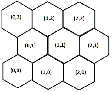
Flat Topped - odd columns shifted up
             _______
            /       \
    _______/  (1,1)  \_______
   /       \         /       \
  /  (0,1)  \_______/  (2,1)  \
  \         /       \         /
   \_______/  (1,0)  \_______/
   /       \         /       \
  /  (0,0)  \_______/  (2,0)  \
  \         /       \         /
   \_______/         \_______/
The column shift changes how we discover nearby nodes. For instance if we take the node at (0,0) and wish to discover the node to its North-East, (1,0), we can simply increment the column value by one.
However if we take the node (1,0) and wish to discover its North-East node at (2,1) we have to increment both the column value and the row value. I.e the calculation changes depending on whether the odd column has been shifted up or down.
In full for a node in an even column we can calculate a nodes neighbours thus:
north      = (column, row + 1)
north-east = (column + 1, row)
south-east = (column + 1, row - 1)
south      = (column, row -1)
south-west = (column - 1, row - 1)
north-west = (column - 1, row)
And for a node in an odd column the node neighbours can be found:
north      = (column, row + 1)
north-east = (column + 1, row + 1)
south-east = (column + 1, row)
south      = (column, row -1)
south-west = (column - 1, row)
north-west = (column - 1, row + 1)
Programmatically these can be found with a public helper function where the grid has boundaries in space denoted by the min and max values, again these ensure that you're not returning nodes outside of your grid area:
pub fn node_neighbours_offset(
    source: (i32, i32),
    orientation: &HexOrientation,
    min_column: i32,
    max_column: i32,
    min_row: i32,
    max_row: i32,
) -> Vec<(i32, i32)>
Where orientation must be HexOrientation::FlatTopOddUp
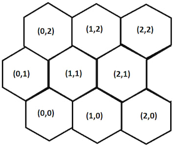
Flat Topped - odd columns shifted down
    _______           _______
   /       \         /       \
  /  (0,1)  \_______/  (2,1)  \
  \         /       \         /
   \_______/  (1,1)  \_______/
   /       \         /       \
  /  (0,0)  \_______/  (2,0)  \
  \         /       \         /
   \_______/  (1,0)  \_______/
           \         /
            \_______/
The column shift changes how we discover nearby nodes. For instance if we take the node at (0,0) and wish to discover the node to its North-East, (1,1), we increment the column and row values by one.
However if we take the node (1,1) and wish to discover its North-East node at (2,1) we have to only increment the column value by one.
In full for a node in an even column we can calculate a nodes neighbours thus:
north      = (column, row + 1)
north-east = (column + 1, row + 1)
south-east = (column + 1, row)
south      = (column, row -1)
south-west = (column - 1, row)
north-west = (column - 1, row + 1)
And for a node in an odd column the node neighbours can be found:
north      = (column, row + 1)
north-east = (column + 1, row)
south-east = (column + 1, row - 1)
south      = (column, row -1)
south-west = (column - 1, row - 1)
north-west = (column - 1, row)
Programmatically these can be found with a public helper function where the grid has boundaries in space denoted by the min and max values:
pub fn node_neighbours_offset(
    source: (i32, i32),
    orientation: &HexOrientation,
    min_column: i32,
    max_column: i32,
    min_row: i32,
    max_row: i32,
) -> Vec<(i32, i32)>
Where orientation must be HexOrientation::FlatTopOddDown
Pointy Top - odd rows shifted right
(Ascii hexagons with pointy tops are very hard to draw so it's time for some MSPaint)
The row shift changes how we discover nearby nodes. For instance if we take the node at (0,0) and wish to discover the node to its North-East, (0,1), we increment the row value by one.
However if we take the node (0,1) and wish to discover its North-East node at (1,2) we have to increment both the column and row values by one.
In full for a node in an even row we can calculate a nodes neighbours thus:
north-east = (column, row + 1)
east       = (column + 1, row)
south-east = (column, row - 1)
south-west = (column - 1, row - 1)
west       = (column -1, row)
north-west = (column - 1, row + 1)
And for a node in an odd row the node neighbours can be found:
north-east = (column + 1, row + 1)
east       = (column + 1, row)
south-east = (column + 1, row - 1)
south-west = (column, row - 1)
west       = (column -1, row)
north-west = (column, row + 1)
Pointy Top - odd rows shifted left
(Ascii hexagons with pointy tops are very hard to draw so it's time for some MSPaint)
The row shift changes how we discover nearby nodes. For instance if we take the node at (0,0) and wish to discover the node to its North-East, (1,1), we increment the column and row values by one.
However if we take the node (1,1) and wish to discover its North-East node at (1,2) we have to increment only the row value by one.
In full for a node in an even row we can calculate a nodes neighbours thus:
north-east = (column + 1, row + 1)
east       = (column + 1, row)
south-east = (column + 1, row - 1)
south-west = (column, row - 1)
west       = (column -1, row)
north-west = (column, row + 1)
And for a node in an odd row the node neighbours can be found:
north-east = (column, row + 1)
east       = (column + 1, row)
south-east = (column, row - 1)
south-west = (column - 1, row - 1)
west       = (column -1, row)
north-west = (column - 1, row + 1)
What Coordinate System Should You Use?
If you're building a square/rectangular grid I'd say the Offset layout is the easiest to begin working with, it is simply just columns and rows on an x-y like axes with a little column/row shifting.
If you're building a circular grid then Axial and Cubic are easily the best as their coordinate systems naturally fit a circular space.
You could use Axial and Cubic for a square/rectangular grid by creating a very large circle and using extremely high complexity values to mark out hexagons in the four edges of the space, however this is just a waste of memory to store and for complex pathfinding the algorithm may wate time probing a corner.
How to use
Cargo.toml
[dependencies]
hexagonal_pathfinding_astar = "1.0"
Offset Exmaple
Part of xyz.rs
use hexagonal_pathfinding_astar::*;
// you are here
let start_node: (i32, i32) = (0, 0);
// keys are nodes, values are your measure of 'complexity' to traverse it
let mut nodes: HashMap<(i32, i32), f32> = HashMap::new();
nodes.insert((0, 0), 1.0);
nodes.insert((0, 1), 1.0);
nodes.insert((0, 2), 1.0);
nodes.insert((0, 3), 3.0);
nodes.insert((1, 0), 2.0);
nodes.insert((1, 1), 9.0);
nodes.insert((1, 2), 4.0);
nodes.insert((1, 3), 2.0);
nodes.insert((2, 0), 2.0);
nodes.insert((2, 1), 6.0);
nodes.insert((2, 2), 8.0);
nodes.insert((2, 3), 9.0);
nodes.insert((3, 0), 3.0);
nodes.insert((3, 1), 4.0);
nodes.insert((3, 2), 5.0);
nodes.insert((3, 3), 2.0);
// you want to go here
let end_node: (i32, i32) = (3, 3);
// the 'exclusive' limit of grid size
let min_column = -1;
let max_column = 4;
let min_row = -1;
let max_row = 4;
// the hexagon arrangement you are using
let orientation = HexOrientation::FlatTopOddUp;
let best = astar_offset::astar_path(start_node, nodes, end_node, min_column, max_column, min_row, max_row, orientation);
// answer using above data = [(0,0), (0,1), (0,2), (1,2), (2,3), (3,3)]
// the manual calculation for this can be found under `docs/calculations_done_manually.md`
Cubic Example
use hexagonal_pathfinding_astar::*;
// you are here
let start_node: (i32, i32, i32) = (0, 0, 0);
// keys are nodes, values are the complexity
let mut nodes: HashMap<(i32, i32, i32), f32> = HashMap::new();
nodes.insert((0, 0, 0), 1.0);
nodes.insert((0, -1, 1), 1.0);
nodes.insert((1, -1, 0), 15.0);
nodes.insert((1, 0, -1), 14.0);
nodes.insert((0, 1, -1), 2.0);
nodes.insert((-1, 1, 0), 6.0);
nodes.insert((-1, 0, 1), 7.0);
nodes.insert((0, -2, 2), 1.0);
nodes.insert((1, -2, 1), 14.0);
nodes.insert((2, -2, 0), 1.0);
nodes.insert((2, -1, -1), 1.0);
nodes.insert((2, 0, -2), 1.0);
nodes.insert((1, 1, -2), 1.0);
nodes.insert((0, 2, -2), 1.0);
nodes.insert((-1, 2, -1), 3.0);
nodes.insert((-2, 2, 0), 1.0);
nodes.insert((-2, 1, 1), 8.0);
nodes.insert((-2, 0, 2), 1.0);
nodes.insert((-1, -1, 2), 2.0);
// you want to go here
let end_node: (i32, i32, i32) = (2, -2, 0);
// it's a circular grid with a limited number of rings
let rings = 2;
let best = astar_cubic::astar_path(start_node, nodes, end_node, rings);
// answer = vec![(0, 0, 0),(0, 1, -1),(1, 1, -2),(2, 0, -2),(2, -1, -1),(2, -2, 0)]