lazyivy

lazyivy is a Rust crate that provides tools to solve initial value problems of the form dY/dt = F(t, Y) using Runge-Kutta methods, where Y is a vector and t is a scalar.

The algorithms are implemented using the struct RungeKutta, that implements Iterator. The following Runge-Kutta methods are implemented currently, and more will be added in the near future.

• Euler 1
• Ralston 2
• Huen-Euler 2(1)
• Bogacki-Shampine 3(2)
• Fehlberg 4(5)
• Dormand-Prince 5(4)

(p is the order of the method and (p*) is the order of the embedded error estimator, if it is present.)

Lazy integration

RungeKutta implements the Iterator trait. Each .next() call advances the iteration to the next Runge-Kutta step and returns a tuple (t, Y), where t is the dependent variable and Y is Array1<f64>.

Note that each Runge-Kutta step contains s number of internal stages. Using lazyivy, there is no way at present to access the integration values for these inner stages. The .next() call returns the final result for each step, summed over all stages.

The lazy implementation of Runge-Kutta means that you can consume the iterator in different ways. For e.g., you can use .last() to keep only the final result, .collect() to gather the state at all steps, .map() to chain the iterator with another, etc. You may also choose to use it in a for loop and implement you own logic for modifying the step-size or customizing the stop condition.

API is unstable. It is active and under development.

Usage:

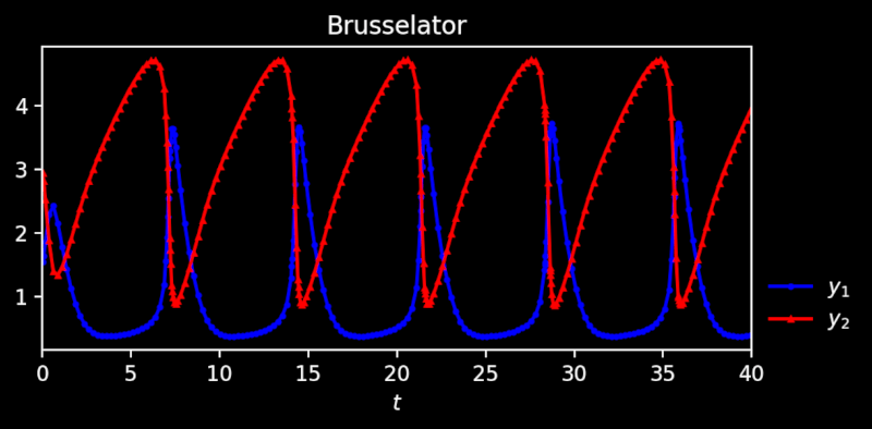
After adding lazyivy to Cargo.toml, create an initial value problem using the provided builder. Here is an example showing how to solve the Brusselator.

\frac{d}{dt} \left[ \begin{array}{c}
 y_1 \\ y_2 \end{array}\right] = \left[\begin{array}{c}1 - y_1^2 y_2 - 4 y_1 
 \\ 3y_1 - y_1^2 y_2 \end{array} \right]

use lazyivy::RungeKutta;
use ndarray::{array, ArrayView1, ArrayViewMut1};
 
 
fn brusselator(_t: &f64, y: ArrayView1<f64>, mut result: ArrayViewMut1<f64>) {
    result[0] = 1. + y[0].powi(2) * y[1] - 4. * y[0];
    reuslt[1] = 3. * y[0] - y[0].powi(2) * y[1];
}
 
fn main() {
    let t0: f64 = 0.;
    let y0 = array![1.5, 3.];
    let absolute_tol = array![1.0e-4, 1.0e-4];
    let relative_tol = array![1.0e-4, 1.0e-4];
 
    // Instantiate a integrator for an ODE system with adaptive step-size 
    // Runge-Kutta. The `builder` method takes in as argument the evaluation
    // function and the predicate function (that determines when to stop). You
    // need to call `build()` to consume the builder and return a `RungeKutta`
    // struct.
 
    let mut integrator = RungeKutta::builder(brusselator, |t, _| *t > 40.)
        .initial_condition(t0, y0)
        .initial_step_size(0.025)
        .method("dormandprince", true)   // `true` for adaptive step-size
        .tolerances(absolute_tol, relative_tol)
        .set_max_step_size(0.25)
        .build()
        .unwrap();
 
    // For adaptive algorithms, you can use this to improve the initial guess 
    // for the step size.
    integrator.set_step_size(&integrator.guess_initial_step());
 
    // Perform the iterations and print each state.
    for item in integrator {
        println!("{:?}", item);   // Prints (t, array[y1, y2]) for each step.
    }
}

The result when plotted looks like this,

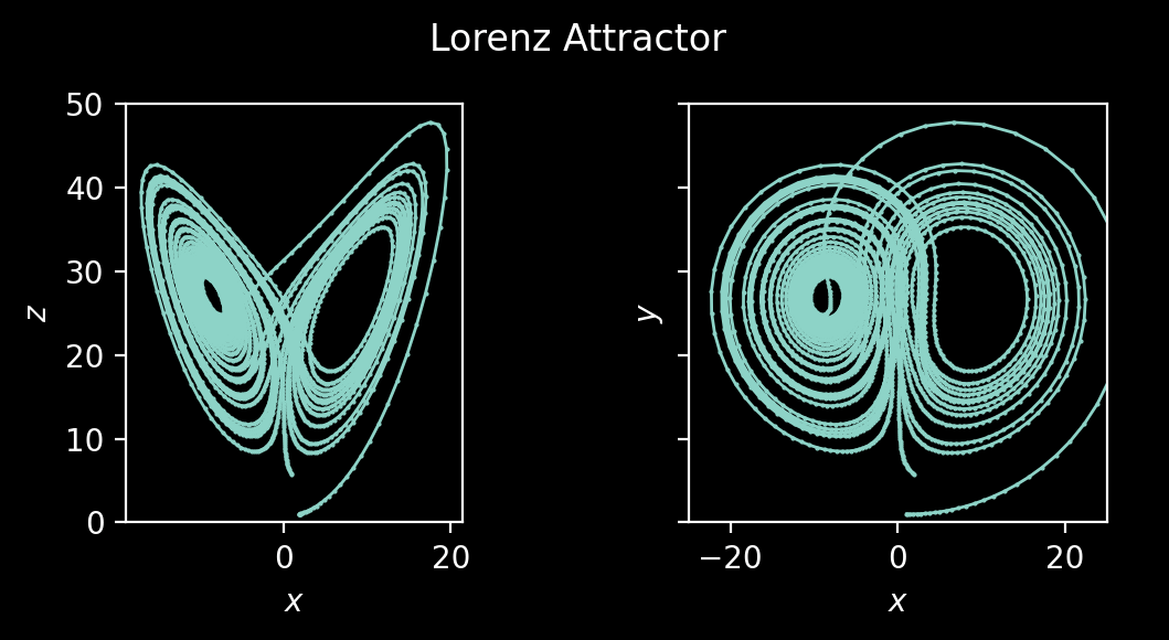
Likewise, you can do the same for other problems, e.g. for the Lorenz attractor, define the evaluation function

fn lorentz_attractor(_t: &f64, y: ArrayView1<f64>, mut result: ArrayViewMut1<f64>) {
    result[0] = 10. * (y[1] - y[0]);
    result[1] = y[0] * (28. - y[2]) - y[1];
    result[2] = y[0] * y[1] - 8. / 3. * y[2];
}

You can also use closures to capture the environment and wrap your evaluation. That is, if you have a function -

fn lorentz_attractor(
    x: f64, 
    y: f64, 
    z: f64, 
    sigma: f64, 
    beta: f64,
    rho: f64
    ) -> Array1<f64> {
    array![
        sigma * (y - x),
        x * (rho - z) - y,
        x * y - beta * z,
    ]
}

you cannot pass this to RungeKutta::builder() directly. But you can wrap this into a closure. E.g.,

let sigma = 10.;
let beta = 8. / 3.;
let rho: 28.;

let eval_closure = |_t, y, result| {    // here result is mut
    // Closure captures the environment and wraps the function signature
    result = lorentz_attractor(y[0], y[1], y[2], sigma, beta, rho);
};

let integrator = RungeKutta::builder(eval_closure, |t, _| *t > 20.)
    ... // other parameters
    .build();

This works because closures that do not modify their environments can coerce to Fn. Hence, this pattern will not work for closures that mutate their environments. In general, you can use any evaluation function and stop condition, but they must be Fn(&f64, ArrayView1<f64>, ArrayViewMut1<f64>) and Fn(&f64, ArrayView1<f64>) -> bool, respectively.

Here is a plot showing the Lorenz attractor result.

Mutating in-place (as of version 0.5.0)

In the above example for the Lorenz attractor, I created a new array using the array! macro. However, I recommend in practice that you use evaluation functions that mutate a result array that is passed to the function.

For example, the same example could take the form -

fn lorentz_attractor(
    x: f64, 
    y: f64, 
    z: f64, 
    sigma: f64, 
    beta: f64,
    rho: f64,
    result: ArrayViewMut1<f64>,   // Mutate this argument in-place.
    ) {
    result[0] = sigma * (y - x);
    result[1] = x * (rho - z) - y;
    result[2] = x * y - beta * z;
}

And then you can wrap this in a closure with the appropriate signature.

let sigma = 10.;
let beta = 8. / 3.;
let rho: 28.;

let eval_closure = |_t, y, result| {    // here result is mut
    lorentz_attractor(y[0], y[1], y[2], sigma, beta, rho, result);
    //                                                    ^-----
    //                                       Added result as an argument
};

This way you will avoid an allocation each time the function is called.

To facilitate this change, as of v0.5.0, the signature of the generic parameter F that was previously Fn(&f64, &Array1<f64>) -> Array1<f64> was changed to Fn(&f64, ArrayView1<f64>, ArrayViewMut1<f64>).

Since Rust does not allow for mutiple mutable references, this change does mean that RungeKutta is no longer thread-safe. But, this should be fine because Runge-Kutta iterations are sequential and cannot easily be multi-threaded.

To-do:

• Add better tests.
• Benchmark.